You're reading the documentation of the v0.6. For the latest released version, please have a look at v1.2.
Perceval Detailed Walkthrough
In this notebook, we aim to reproduce the \(\mathsf{CNOT}\) Gate to evaluate its performance while demonstrating key features of Perceval. We use as basis the implementation from [1].
[1]:
import perceval as pcvl
import perceval.lib.phys as phys
import sympy as sp
import numpy as np
Ralph CNOT Gate
We start by describing the circuit as defined by the paper above- it is a circuit on six modes (labelled from 0 to 5 from top to bottom) consisting of five beam splitters. Modes 1 and 2 contain the control system while modes 3 and 4 encode the target syestem. Modes 0 and 5 are unoccupied ancillary modes.
[2]:
cnot = phys.Circuit(6, name="Ralph CNOT")
cnot.add((0, 1), phys.BS(R=1/3, phi_b=sp.pi, phi_d=0))
cnot.add((3, 4), phys.BS(R=1/2))
cnot.add((2, 3), phys.BS(R=1/3, phi_b=sp.pi, phi_d=0))
cnot.add((4, 5), phys.BS(R=1/3))
cnot.add((3, 4), phys.BS(R=1/2))
pcvl.pdisplay(cnot)
We can then simulate this circuit using the Naive backend on four different input states corresponding to the two-qubit computational basis states. We use CircuitAnalyser to analyse the performance of the gate.
[3]:
simulator_backend = pcvl.BackendFactory().get_backend("Naive")
s_cnot = simulator_backend(cnot.U)

states = {
    pcvl.BasicState([0, 1, 0, 1, 0, 0]): "00",
    pcvl.BasicState([0, 1, 0, 0, 1, 0]): "01",
    pcvl.BasicState([0, 0, 1, 1, 0, 0]): "10",
    pcvl.BasicState([0, 0, 1, 0, 1, 0]): "11"
}

ca = pcvl.CircuitAnalyser(s_cnot, states)
ca.compute(expected={"00": "00", "01": "01", "10": "11", "11": "10"})
pcvl.pdisplay(ca)
print("performance=%s, error rate=%.3f%%" % (pcvl.simple_float(ca.performance)[1], ca.error_rate))
| 00 | 01 | 10 | 11 | |
|---|---|---|---|---|
| 00 | 0.999991 | 0 | 0 | 0 |
| 01 | 0 | 0.999991 | 0 | 0 |
| 10 | 0 | 0 | 0 | 0.999991 |
| 11 | 0 | 0 | 0.999991 | 0 |
performance=1/9, error rate=0.000%
Beyond the actual logic function, what is interesting with this gate us that it produces entangled states that we will be trying to check with CHSH experiment when the source is not perfect.
Checking for entanglement with CHSH experiment
 https://en.wikipedia.org/wiki/File:Two_channel_bell_test.svg
To reproduce this Bell test protocol, we define a new circuit which uses the \(\mathsf{CNOT}\) gate implemented above as a sub-circuit. The parameters \(a\) and \(b\) describe the measurement bases used by players \(A\) and \(B\) in the runs of the Bell-test.
[4]:
test_cnot = phys.Circuit(6)
test_cnot.add((1, 2), phys.BS())

test_cnot //= cnot

a = pcvl.Parameter("a")
b = pcvl.Parameter("b")

test_cnot.add((1, 2), phys.BS(theta=a))
test_cnot.add((3, 4), phys.BS(theta=b))

pcvl.pdisplay(test_cnot)
We start by setting the values of the two parameters to 0, meaning that the beam splitters after the \(\mathsf{CNOT}\) effectively act as the identity.
[5]:
a.set_value(0)
b.set_value(0)
We now define a photon source with a brightness of 40% and a purity of 99%. We then define a Processor which plugs two such sources to the circuit above, on ports 2 and 3 (using the 0-index convention).
[6]:
source = pcvl.Source(brightness=0.40, purity=0.99)
QPU = pcvl.Processor({2:source, 3:source}, test_cnot)
We now detail the different state vectors that are the probabilistic inputs to the circuit. The most frequent input is the empty state, followed by two states with only a single photon on either of the input ports, then by the expected nominal input \(|0,0,1,1,0,0\rangle\).
[7]:
pcvl.pdisplay(QPU.source_distribution, precision=1e-4)
| state | probability |
|---|---|
| |0,0,0,0,0,0> | 9/25 |
| |0,0,0,1,0,0> | 0.2376 |
| |0,0,1,0,0,0> | 0.2376 |
| |0,0,1,1,0,0> | 0.1568 |
| |0,0,0,2,0,0> | 0.0024 |
| |0,0,2,0,0,0> | 0.0024 |
| |0,0,2,1,0,0> | 0.0016 |
| |0,0,1,2,0,0> | 0.0016 |
| |0,0,2,2,0,0> | 0 |
We can then check the output state distribution corresponding to this input distribution.
[8]:
_, output_distribution=QPU.run(simulator_backend)
pcvl.pdisplay(output_distribution, max_v=10)
| state | probability |
|---|---|
| |0,0,0,0,0,0> | 0.360006 |
| |0,0,0,1,0,0> | 0.118802 |
| |0,0,1,0,0,0> | 0.118802 |
| |0,0,0,0,0,1> | 0.079201 |
| |1,0,0,0,0,0> | 0.079201 |
| |0,0,0,0,1,0> | 0.039601 |
| |0,1,0,0,0,0> | 0.039601 |
| |0,0,2,0,0,0> | 0.017758 |
| |0,0,0,2,0,0> | 0.017758 |
| |1,0,1,0,0,0> | 0.017691 |
Let us run now the experiment with decreasing value of purity in the range \([0.98,1]\) and check the CHSH inequality.
[9]:
from tqdm.auto import tqdm
x = np.arange(0, 2, 0.05)
y = []

for imp in tqdm(x):
    Es = []
    for va in [0, sp.pi/4]:
        a.set_value(va)
        for vb in [sp.pi/8, 3*sp.pi/8]:
            b.set_value(vb)
            Npp, Npm, Nmp, Nmm = 0, 0, 0, 0
            source = pcvl.Source(brightness=0.15, purity=1-imp/100)
            # we add a post-selection on the processor, there needs to be zero photon in the ancilla modes 1,6
            # and exactly one in mode 2,3 and one in mode 3,4
            QPU = pcvl.Processor({2:source, 3:source},
                                 test_cnot, lambda o: o[0]==0 and (o[1]+o[2]==1) and (o[3]+o[4]==1) and o[5]==0)
            _, output_distribution=QPU.run(simulator_backend)
            for output_sv, prob in output_distribution.items():
                output_state = output_sv[0]
                if (output_state[1] == 1 and output_state[3] == 1):
                    Npp = prob
                if (output_state[1] == 1 and output_state[4] == 1):
                    Npm = prob
                if (output_state[2] == 1 and output_state[3] == 1):
                    Nmp = prob
                if (output_state[2] == 1 and output_state[4] == 1):
                    Nmm = prob
            E = (Npp-Npm-Nmp+Nmm)/(Npp+Npm+Nmp+Nmm)
            Es.append(E)

    S = Es[0]-Es[1]+Es[2]+Es[3]
    print("purity=",1-imp/100, "S=", S)
    y.append(S)
purity= 1.0 S= 2.8284271247461903
purity= 0.9995 S= 2.7808356540538646
purity= 0.999 S= 2.734207894156242
purity= 0.9985 S= 2.688514934096702
purity= 0.998 S= 2.6437290078861326
purity= 0.9975 S= 2.599823438378157
purity= 0.997 S= 2.5567725844135643
purity= 0.9965 S= 2.5145517910141844
purity= 0.996 S= 2.4731373424226386
purity= 0.9955 S= 2.43250641780031
purity= 0.995 S= 2.39263704940936
purity= 0.9945 S= 2.353508083118063
purity= 0.994 S= 2.3150991410799877
purity= 0.9935 S= 2.2773905864489574
purity= 0.993 S= 2.240363490001148
purity= 0.9925 S= 2.203999598545389
purity= 0.992 S= 2.1682813050106335
purity= 0.9915 S= 2.1331916201078847
purity= 0.991 S= 2.0987141454704625
purity= 0.9905 S= 2.0648330481836887
purity= 0.99 S= 2.0315330366205884
purity= 0.9895 S= 1.9987993375063846
purity= 0.989 S= 1.9666176741392758
purity= 0.9885 S= 1.9349742457002677
purity= 0.988 S= 1.9038557075888374
purity= 0.9875 S= 1.8732491527257937
purity= 0.987 S= 1.8431420937680647
purity= 0.9865 S= 1.813522446184165
purity= 0.986 S= 1.7843785121419113
purity= 0.9855 S= 1.7556989651634898
purity= 0.985 S= 1.7274728355053663
purity= 0.9845 S= 1.6996894962236047
purity= 0.984 S= 1.6723386498871988
purity= 0.9835 S= 1.6454103159047264
purity= 0.983 S= 1.6188948184313598
purity= 0.9825 S= 1.592782774825639
purity= 0.982 S= 1.5670650846268965
purity= 0.9815 S= 1.541732919026313
purity= 0.981 S= 1.516777710805831
purity= 0.9805 S= 1.4921911447210179
[10]:
import matplotlib.pyplot as plt
plt.title("CHSH value with purity")
plt.xlabel("impurity (%)")
plt.ylabel("bell inegality")
plt.axhline(y=2, linewidth=2, color="red", label= 'horizontal-line')
plt.plot(x, y, color ="green")
plt.grid(color='b', dashes=(3, 2, 1, 2))
plt.show()
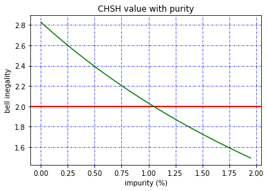
Beyond only 1% of impurity, we are crossing the value \(2\), ie not violating anymore the \(|CHSH|\le 2\) inegality!
Reference
[1] T. C. Ralph, N. K. Langford, T. B. Bell, and A. G. White. Linear optical controlled-NOT gate in the coincidence basis. Physical Review A, 65(6):062324, June 2002. Publisher: American Physical Society.