You're reading the documentation of the v0.6. For the latest released version, please have a look at v1.2.
Variational Quantum Eigensolver
We provide a Perceval implementation of original photonic Variational Quantum Eigensolver (VQE) from Peruzzo, A. et al. in [1].
This notebook provides computations of ground-state molecular energies for the Hamiltonian given by the following papers:
\(\bullet\) A variational eigenvalue solver on a photonic quantum processor [1].
\(\bullet\) Scalable Quantum Simulation of Molecular Energies [2] .
\(\bullet\) Computation of Molecular Spectra on a Quantum Processor with an Error-Resilient Algorithm [3]
Importing the necessary packages for the computations:
[1]:
from IPython import display
from collections import Counter
from tabulate import tabulate
from tqdm.auto import tqdm

import perceval as pcvl
import quandelibc as qc
import perceval.lib.phys as phys
import perceval.lib.symb as symb

import math as math
import numpy.polynomial.polynomial as nppol
import sympy as sp
import numpy as np
from scipy.optimize import minimize
import random
import matplotlib.pyplot as plt
simulator_backend = pcvl.BackendFactory().get_backend("Naive")
Implementation in Perceval
Here we reproduce on Perceval the 2-qubit circuit used in [1] for VQE.
We use path encoded qubits.
Modes 0 and 5 are auxillary. 1\(^\text{st}\) qubit is path encoded in modes 1 and 2. 2\(^\text{nd}\) qubit in modes 3 and 4.
[2]:
#List of the parameters φ1,φ2,...,φ8
List_Parameters=[]

# VQE is a 6 optical mode circuit
VQE=pcvl.Circuit(6)

VQE.add((1,2), phys.BS(R=1/2))
VQE.add((3,4), phys.BS(R=1/2))
List_Parameters.append(pcvl.Parameter("φ1"))
VQE.add((2,),phys.PS(phi=List_Parameters[-1]))
List_Parameters.append(pcvl.Parameter("φ3"))
VQE.add((4,),phys.PS(phi=List_Parameters[-1]))
VQE.add((1,2), phys.BS(R=1/2))
VQE.add((3,4), phys.BS(R=1/2))
List_Parameters.append(pcvl.Parameter("φ2"))
VQE.add((2,),phys.PS(phi=List_Parameters[-1]))
List_Parameters.append(pcvl.Parameter("φ4"))
VQE.add((4,),phys.PS(phi=List_Parameters[-1]))


# CNOT ( Post-selected with a success probability of 1/9)
VQE.add([0,1,2,3,4,5], phys.PERM([0,1,2,3,4,5]))#Identity PERM (permutation) for the purpose of drawing a nice circuit
VQE.add((3,4), phys.BS(R=1/2))
VQE.add([0,1,2,3,4,5], phys.PERM([0,1,2,3,4,5]))#Identity PERM (permutation) for the same purpose
VQE.add((0,1), phys.BS(R=1/3))
VQE.add((2,3), phys.BS(R=1/3))
VQE.add((4,5), phys.BS(R=1/3))
VQE.add([0,1,2,3,4,5], phys.PERM([0,1,2,3,4,5]))#Identity PERM (permutation) for the same purpose
VQE.add((3,4), phys.BS(R=1/2))
VQE.add([0,1,2,3,4,5], phys.PERM([0,1,2,3,4,5]))#Identity PERM (permutation) for the same purpose

List_Parameters.append(pcvl.Parameter("φ5"))
VQE.add((2,),phys.PS(phi=List_Parameters[-1]))
List_Parameters.append(pcvl.Parameter("φ7"))
VQE.add((4,),phys.PS(phi=List_Parameters[-1]))
VQE.add((1,2), phys.BS(R=1/2))
VQE.add((3,4), phys.BS(R=1/2))
List_Parameters.append(pcvl.Parameter("φ6"))
VQE.add((2,),phys.PS(phi=List_Parameters[-1]))
List_Parameters.append(pcvl.Parameter("φ8"))
VQE.add((4,),phys.PS(phi=List_Parameters[-1]))
VQE.add((1,2), phys.BS(R=1/2))
VQE.add((3,4), phys.BS(R=1/2))

# Mode 0 and 5 are auxillary.
#1st qubit is path encoded in modes 1 & 2
#2nd qubit in 3 & 4

print("The circuit is :")
pcvl.pdisplay(VQE)
The circuit is :
Logical input and output states
Logical states are path encoded on the Fock States.
[3]:
#Input states of the photonic circuit
input_states = {
    pcvl.BasicState([0,1,0,1,0,0]):"|00>"}

#Outputs in the computational basis
output_states = {
    pcvl.BasicState([0,1,0,1,0,0]):"|00>",
    pcvl.BasicState([0,1,0,0,1,0]):"|01>",
    pcvl.BasicState([0,0,1,1,0,0]):"|10>",
    pcvl.BasicState([0,0,1,0,1,0]):"|11>"}
Loss function for the variational algorithm
For a given state \(|\psi \rangle\) the Rayleigh-Ritz quotient is given by:
This is computed in Perceval by explicitly computing \(|\psi \rangle\) ( which is the output of the simulated photonic circuit). Determining the smallest/ground state eigenvalue is done through a variational approach with Rayleigh-Ritz quotient as the loss function.
Using a classical optimisation algorithm, and the simulations given by Perceval we find the eigenvector which minimises the Rayleigh-Ritz quotient together with its associated eigenvalue ( the ground state eigenvalue), which reprensents the solution of the VQE.
[4]:
def minimize_loss(lp=None):
    # Updating the parameters on the chip
    for idx, p in enumerate(lp):
        List_Parameters[idx].set_value(p)

    #Simulation, Quantum processing part of the VQE
    s_VQE = simulator_backend(VQE.compute_unitary(use_symbolic = False))

    # Collecting the output state of the circuit
    psi = []
    for input_state in input_states:
        for output_state in output_states: #|00>,|01>,|10>,|11>
            psi.append(s_VQE.probampli(input_state,output_state))

        #Evaluating the mean value of the Hamiltonian.  # The Hamiltonians H is defined in the following block
    psi_prime=np.dot(H[R][1],psi)
    loss = np.real(sum(sum(np.conjugate(psi)*np.array(psi_prime[0]))))/(sum([i*np.conjugate(i) for i in psi]))
    loss=np.real(loss)

    tq.set_description('%g / %g  loss function=%g' % (R, len(H), loss))
    return(loss)
Hamiltonians for VQE
In this section we define the 3 Hamiltonians given by the 3 papers [1-3]
Perceval can compute the state vector, which is the output of the photonic quantum circuit, explicitly. This eliminates the need for using algorithms to estimate the expectation value.
A Hamiltonian can be written as :
where \(h_{\sigma} \in \mathbb{R}\) and \(\sigma\) are pauli operators.
Hamiltonian n°1 [1]
Hamiltonian coefficents on the supplementary paper:
[8]:
Hamiltonian_elem = np.array([[[0,0,0,0],[0,0,0,0],[0,0,0,0],[0,0,0,0]],    #00
                             [[1,0,0,0],[0,1,0,0],[0,0,1,0],[0,0,0,1]],    #II
                             [[0,1,0,0],[1,0,0,0],[0,0,0,1],[0,0,1,0]],    #IX
                             [[1,0,0,0],[0,-1,0,0],[0,0,1,0],[0,0,0,-1]],  #IZ
                             [[0,0,1,0],[0,0,0,1],[1,0,0,0],[0,1,0,0]],    #XI
                             [[0,0,0,1],[0,0,1,0],[0,1,0,0],[1,0,0,0]],    #XX
                             [[0,0,1,0],[0,0,0,-1],[1,0,0,0],[0,-1,0,0]],  #XZ
                             [[1,0,0,0],[0,1,0,0],[0,0,-1,0],[0,0,0,-1]],  #ZI
                             [[0,1,0,0],[1,0,0,0],[0,0,0,-1],[0,0,-1,0]],  #ZX
                             [[1,0,0,0],[0,-1,0,0],[0,0,-1,0],[0,0,0,1]]]) #ZZ


Hamiltonian_coef = np.matrix(
# [R,II,IX,IZ,XI,XZ,XX,ZI,ZX,ZZ]
[[0.05,33.9557,-0.1515,-2.4784,-0.1515,0.1412,0.1515,-2.4784,0.1515,0.2746],
[0.1,13.3605,-0.1626,-2.4368,-0.1626,0.2097,0.1626,-2.4368,0.1626,0.2081],
[0.15,6.8232,-0.1537,-2.3801,-0.1537,0.2680,0.1537,-2.3801,0.1537,0.1512],
[0.2,3.6330,-0.1405,-2.2899,-0.1405,0.3027,0.1405,-2.2899,0.1405,0.1176],
[0.25,1.7012,-0.1324,-2.1683,-0.1324,0.3211,0.1324,-2.1683,0.1324,0.1010],
[0.3,0.3821,-0.1306,-2.0305,-0.1306,0.3303,0.1306,-2.0305,0.1306,0.0943],
[0.35,-0.5810,-0.1335,-1.8905,-0.1335,0.3344,0.1335,-1.8905,0.1335,0.0936],
[0.4,-1.3119,-0.1396,-1.7568,-0.1396,0.3352,0.1396,-1.7568,0.1396,0.0969],
[0.45,-1.8796,-0.1477,-1.6339,-0.1477,0.3339,0.1477,-1.6339,0.1477,0.1030],
[0.5,-2.3275,-0.1570,-1.5236,-0.1570,0.3309,0.1570,-1.5236,0.1570,0.1115],
[0.55,-2.6844,-0.1669,-1.4264,-0.1669,0.3264,0.1669,-1.4264,0.1669,0.1218],
[0.6,-2.9708,-0.1770,-1.3418,-0.1770,0.3206,0.1770,-1.3418,0.1770,0.1339],
[0.65,-3.2020,-0.1871,-1.2691,-0.1871,0.3135,0.1871,-1.2691,0.1871,0.1475],
[0.7,-3.3893,-0.1968,-1.2073,-0.1968,0.3052,0.1968,-1.2073,0.1968,0.1626],
[0.75,-3.5417,-0.2060,-1.1552,-0.2060,0.2958,0.2060,-1.1552,0.2060,0.1791],
[0.8,-3.6660,-0.2145,-1.1117,-0.2145,0.2853,0.2145,-1.1117,0.2145,0.1968],
[0.85,-3.7675,-0.2222,-1.0758,-0.2222,0.2738,0.2222,-1.0758,0.2222,0.2157],
[0.9,-3.8505,-0.2288,-1.0466,-0.2288,0.2613,0.2288,-1.0466,0.2288,0.2356],
[0.95,-3.9183,-0.2343,-1.0233,-0.2343,0.2481,0.2343,-1.0233,0.2343,0.2564],
[1,-3.9734,-0.2385,-1.0052,-0.2385,0.2343,0.2385,-1.0052,0.2385,0.2779],
[1.05,-4.0180,-0.2414,-0.9916,-0.2414,0.2199,0.2414,-0.9916,0.2414,0.3000],
[1.1,-4.0539,-0.2430,-0.9820,-0.2430,0.2053,0.2430,-0.9820,0.2430,0.3225],
[1.15,-4.0825,-0.2431,-0.9758,-0.2431,0.1904,0.2431,-0.9758,0.2431,0.3451],
[1.2,-4.1050,-0.2418,-0.9725,-0.2418,0.1756,0.2418,-0.9725,0.2418,0.3678],
[1.25,-4.1224,-0.2392,-0.9716,-0.2392,0.1610,0.2392,-0.9716,0.2392,0.3902],
[1.3,-4.1356,-0.2353,-0.9728,-0.2353,0.1466,0.2353,-0.9728,0.2353,0.4123],
[1.35,-4.1454,-0.2301,-0.9757,-0.2301,0.1327,0.2301,-0.9757,0.2301,0.4339],
[1.4,-4.1523,-0.2239,-0.9798,-0.2239,0.1194,0.2239,-0.9798,0.2239,0.4549],
[1.45,-4.1568,-0.2167,-0.9850,-0.2167,0.1068,0.2167,-0.9850,0.2167,0.4751],
[1.5,-4.1594,-0.2086,-0.9910,-0.2086,0.0948,0.2086,-0.9910,0.2086,0.4945],
[1.55,-4.1605,-0.1998,-0.9975,-0.1998,0.0837,0.1998,-0.9975,0.1998,0.5129],
[1.6,-4.1602,-0.1905,-1.0045,-0.1905,0.0734,0.1905,-1.0045,0.1905,0.5304],
[1.65,-4.1589,-0.1807,-1.0116,-0.1807,0.0640,0.1807,-1.0116,0.1807,0.5468],
[1.7,-4.1568,-0.1707,-1.0189,-0.1707,0.0555,0.1707,-1.0189,0.1707,0.5622],
[1.75,-4.1540,-0.1605,-1.0262,-0.1605,0.0479,0.1605,-1.0262,0.1605,0.5766],
[1.8,-4.1508,-0.1503,-1.0334,-0.1503,0.0410,0.1503,-1.0334,0.1503,0.5899],
[1.85,-4.1471,-0.1403,-1.0404,-0.1403,0.0350,0.1403,-1.0404,0.1403,0.6023],
[1.9,-4.1431,-0.1305,-1.0473,-0.1305,0.0297,0.1305,-1.0473,0.1305,0.6138],
[1.95,-4.1390,-0.1210,-1.0540,-0.1210,0.0251,0.1210,-1.0540,0.1210,0.6244],
[2,-4.1347,-0.1119,-1.0605,-0.1119,0.0212,0.1119,-1.0605,0.1119,0.6342],
[2.05,-4.1303,-0.1031,-1.0667,-0.1031,0.0178,0.1031,-1.0667,0.1031,0.6432],
[2.1,-4.1258,-0.0949,-1.0727,-0.0949,0.0148,0.0949,-1.0727,0.0949,0.6516],
[2.15,-4.1214,-0.0871,-1.0785,-0.0871,0.0124,0.0871,-1.0785,0.0871,0.6594],
[2.2,-4.1169,-0.0797,-1.0840,-0.0797,0.0103,0.0797,-1.0840,0.0797,0.6666],
[2.25,-4.1125,-0.0729,-1.0893,-0.0729,0.0085,0.0729,-1.0893,0.0729,0.6733],
[2.3,-4.1082,-0.0665,-1.0944,-0.0665,0.0070,0.0665,-1.0944,0.0665,0.6796],
[2.35,-4.1040,-0.0606,-1.0993,-0.0606,0.0058,0.0606,-1.0993,0.0606,0.6854],
[2.4,-4.0998,-0.0551,-1.1040,-0.0551,0.0047,0.0551,-1.1040,0.0551,0.6909],
[2.45,-4.0957,-0.0500,-1.1085,-0.0500,0.0039,0.0500,-1.1085,0.0500,0.6961],
[2.5,-4.0918,-0.0454,-1.1128,-0.0454,0.0032,0.0454,-1.1128,0.0454,0.7010],
[2.55,-4.0879,-0.0411,-1.1170,-0.0411,0.0026,0.0411,-1.1170,0.0411,0.7056],
[2.6,-4.0841,-0.0371,-1.1210,-0.0371,0.0021,0.0371,-1.1210,0.0371,0.7099],
[2.65,-4.0805,-0.0335,-1.1248,-0.0335,0.0017,0.0335,-1.1248,0.0335,0.7141],
[2.7,-4.0769,-0.0303,-1.1285,-0.0303,0.0014,0.0303,-1.1285,0.0303,0.7181],
[2.75,-4.0735,-0.0273,-1.1321,-0.0273,0.0011,0.0273,-1.1321,0.0273,0.7218],
[2.8,-4.0701,-0.0245,-1.1356,-0.0245,0.0009,0.0245,-1.1356,0.0245,0.7254],
[2.85,-4.0669,-0.0221,-1.1389,-0.0221,0.0007,0.0221,-1.1389,0.0221,0.7289],
[2.9,-4.0638,-0.0198,-1.1421,-0.0198,0.0006,0.0198,-1.1421,0.0198,0.7322],
[2.95,-4.0607,-0.0178,-1.1452,-0.0178,0.0005,0.0178,-1.1452,0.0178,0.7354],
[3,-4.0578,-0.0159,-1.1482,-0.0159,0.0004,0.0159,-1.1482,0.0159,0.7385],
[3.05,-4.0549,-0.0142,-1.1511,-0.0142,0.0003,0.0142,-1.1511,0.0142,0.7414],
[3.1,-4.0521,-0.0127,-1.1539,-0.0127,0.0002,0.0127,-1.1539,0.0127,0.7443],
[3.15,-4.0494,-0.0114,-1.1566,-0.0114,0.0002,0.0114,-1.1566,0.0114,0.7470],
[3.2,-4.0468,-0.0101,-1.1592,-0.0101,0.0001,0.0101,-1.1592,0.0101,0.7497],
[3.25,-4.0443,-0.0090,-1.1618,-0.0090,0.0001,0.0090,-1.1618,0.0090,0.7522],
[3.3,-4.0418,-0.0081,-1.1643,-0.0081,0.0001,0.0081,-1.1643,0.0081,0.7547],
[3.35,-4.0394,-0.0072,-1.1666,-0.0072,0.0001,0.0072,-1.1666,0.0072,0.7571],
[3.4,-4.0371,-0.0064,-1.1690,-0.0064,0.0001,0.0064,-1.1690,0.0064,0.7595],
[3.45,-4.0349,-0.0056,-1.1712,-0.0056,0.0000,0.0056,-1.1712,0.0056,0.7617],
[3.5,-4.0327,-0.0050,-1.1734,-0.0050,0.0000,0.0050,-1.1734,0.0050,0.7639],
[3.55,-4.0306,-0.0044,-1.1756,-0.0044,0.0000,0.0044,-1.1756,0.0044,0.7661],
[3.6,-4.0285,-0.0039,-1.1776,-0.0039,0.0000,0.0039,-1.1776,0.0039,0.7681],
[3.65,-4.0265,-0.0035,-1.1796,-0.0035,0.0000,0.0035,-1.1796,0.0035,0.7702],
[3.7,-4.0245,-0.0030,-1.1816,-0.0030,0.0000,0.0030,-1.1816,0.0030,0.7721],
[3.75,-4.0226,-0.0027,-1.1835,-0.0027,0.0000,0.0027,-1.1835,0.0027,0.7740],
[3.8,-4.0208,-0.0024,-1.1854,-0.0024,0.0000,0.0024,-1.1854,0.0024,0.7759],
[3.85,-4.0190,-0.0021,-1.1872,-0.0021,0.0000,0.0021,-1.1872,0.0021,0.7777],
[3.9,-4.0172,-0.0018,-1.1889,-0.0018,0.0000,0.0018,-1.1889,0.0018,0.7795],
[3.95,-4.0155,-0.0016,-1.1906,-0.0016,0.0000,0.0016,-1.1906,0.0016,0.7812]]
)


#Building the Hamiltonian H[0]= Radius, H[1]=H(Radius)
H1=[]
(n,m)=Hamiltonian_coef.shape
for i in range(n): #i = Radius
    h_0=1.0*np.matrix(Hamiltonian_elem[0])
    for j in range(1,m):
        h_0+= Hamiltonian_coef[i,j]*np.matrix(Hamiltonian_elem[j])
    H1.append([Hamiltonian_coef[i,0],h_0])
Hamiltonian n°2 [2]
[6]:
Hamiltonian_elem = np.array([[[0,0,0,0],[0,0,0,0],[0,0,0,0],[0,0,0,0]],       #00
                             [[1,0,0,0],[0,1,0,0],[0,0,1,0],[0,0,0,1]],       #II
                             [[1,0,0,0],[0,1,0,0],[0,0,-1,0],[0,0,0,-1]],     #ZI
                             [[1,0,0,0],[0,-1,0,0],[0,0,1,0],[0,0,0,-1]],     #IZ
                             [[1,0,0,0],[0,-1,0,0],[0,0,-1,0],[0,0,0,1]],     #ZZ
                             [[0,0,0,1],[0,0,1,0],[0,1,0,0],[1,0,0,0]],       #XX
                             [[0,0,0,-1],[0,0,1,0],[0,1,0,0],[-1,0,0,0]]])    #YY


Hamiltonian_coef = np.matrix(
# [R,II,ZI,IZ,ZZ,XX,YY]
[[0.20,2.8489,0.5678,-1.4508,0.6799,0.0791,0.0791],
[0.25,2.1868,0.5449,-1.2870,0.6719,0.0798,0.0798],
[0.30,1.7252,0.5215,-1.1458,0.6631,0.0806,0.0806],
[0.35,1.3827,0.4982,-1.0226,0.6537,0.0815,0.0815],
[0.40,1.1182,0.4754,-0.9145,0.6438,0.0825,0.0825],
[0.45,0.9083,0.4534,-0.8194,0.6336,0.0835,0.0835],
[0.50,0.7381,0.4325,-0.7355,0.6233,0.0846,0.0846],
[0.55,0.5979,0.4125,-0.6612,0.6129,0.0858,0.0858],
[0.60,0.4808,0.3937,-0.5950,0.6025,0.0870,0.0870],
[0.65,0.3819,0.3760,-0.5358,0.5921,0.0883,0.0883],
[0.70,0.2976,0.3593,-0.4826,0.5818,0.0896,0.0896],
[0.75,0.2252,0.3435,-0.4347,0.5716,0.0910,0.0910],
[0.80,0.1626,0.3288,-0.3915,0.5616,0.0925,0.0925],
[0.85,0.1083,0.3149,-0.3523,0.5518,0.0939,0.0939],
[0.90,0.0609,0.3018,-0.3168,0.5421,0.0954,0.0954],
[0.95,0.0193,0.2895,-0.2845,0.5327,0.0970,0.0970],
[1.00,-0.0172,0.2779,-0.2550,0.5235,0.0986,0.0986],
[1.05,-0.0493,0.2669,-0.2282,0.5146,0.1002,0.1002],
[1.10,-0.0778,0.2565,-0.2036,0.5059,0.1018,0.1018],
[1.15,-0.1029,0.2467,-0.1810,0.4974,0.1034,0.1034],
[1.20,-0.1253,0.2374,-0.1603,0.4892,0.1050,0.1050],
[1.25,-0.1452,0.2286,-0.1413,0.4812,0.1067,0.1067],
[1.30,-0.1629,0.2203,-0.1238,0.4735,0.1083,0.1083],
[1.35,-0.1786,0.2123,-0.1077,0.4660,0.1100,0.1100],
[1.40,-0.1927,0.2048,-0.0929,0.4588,0.1116,0.1116],
[1.45,-0.2053,0.1976,-0.0792,0.4518,0.1133,0.1133],
[1.50,-0.2165,0.1908,-0.0666,0.4451,0.1149,0.1149],
[1.55,-0.2265,0.1843,-0.0549,0.4386,0.1165,0.1165],
[1.60,-0.2355,0.1782,-0.0442,0.4323,0.1181,0.1181],
[1.65,-0.2436,0.1723,-0.0342,0.4262,0.1196,0.1196],
[1.70,-0.2508,0.1667,-0.0251,0.4204,0.1211,0.1211],
[1.75,-0.2573,0.1615,-0.0166,0.4148,0.1226,0.1226],
[1.80,-0.2632,0.1565,-0.0088,0.4094,0.1241,0.1241],
[1.85,-0.2684,0.1517,-0.0015,0.4042,0.1256,0.1256],
[1.90,-0.2731,0.1472,0.0052,0.3992,0.1270,0.1270],
[1.95,-0.2774,0.1430,0.0114,0.3944,0.1284,0.1284],
[2.00,-0.2812,0.1390,0.0171,0.3898,0.1297,0.1297],
[2.05,-0.2847,0.1352,0.0223,0.3853,0.1310,0.1310],
[2.10,-0.2879,0.1316,0.0272,0.3811,0.1323,0.1323],
[2.15,-0.2908,0.1282,0.0317,0.3769,0.1335,0.1335],
[2.20,-0.2934,0.1251,0.0359,0.3730,0.1347,0.1347],
[2.25,-0.2958,0.1221,0.0397,0.3692,0.1359,0.1359],
[2.30,-0.2980,0.1193,0.0432,0.3655,0.1370,0.1370],
[2.35,-0.3000,0.1167,0.0465,0.3620,0.1381,0.1381],
[2.40,-0.3018,0.1142,0.0495,0.3586,0.1392,0.1392],
[2.45,-0.3035,0.1119,0.0523,0.3553,0.1402,0.1402],
[2.50,-0.3051,0.1098,0.0549,0.3521,0.1412,0.1412],
[2.55,-0.3066,0.1078,0.0572,0.3491,0.1422,0.1422],
[2.60,-0.3079,0.1059,0.0594,0.3461,0.1432,0.1432],
[2.65,-0.3092,0.1042,0.0614,0.3433,0.1441,0.1441],
[2.70,-0.3104,0.1026,0.0632,0.3406,0.1450,0.1450],
[2.75,-0.3115,0.1011,0.0649,0.3379,0.1458,0.1458],
[2.80,-0.3125,0.0997,0.0665,0.3354,0.1467,0.1467],
[2.85,-0.3135,0.0984,0.0679,0.3329,0.1475,0.1475]]

)


#Building the Hamiltonian H[0]= Radius, H[1]=H(Radius)
H2=[]
(n,m)=Hamiltonian_coef.shape
for i in range(n): #i = Radius
    h_0=1.0*np.matrix(Hamiltonian_elem[0])
    for j in range(1,m):
        h_0+= Hamiltonian_coef[i,j]*np.matrix(Hamiltonian_elem[j])
    H2.append([Hamiltonian_coef[i,0],h_0])
Hamiltonian n°3 [3]
Hamiltonian coefficents on the supplementary material.
[7]:
Hamiltonian_elem = np.array([[[0,0,0,0],[0,0,0,0],[0,0,0,0],[0,0,0,0]],      #00
                             [[1,0,0,0],[0,1,0,0],[0,0,1,0],[0,0,0,1]],      #II
                             [[1,0,0,0],[0,1,0,0],[0,0,-1,0],[0,0,0,-1]],    #ZI
                             [[0,0,0,1],[0,0,1,0],[0,1,0,0],[1,0,0,0]],      #XX
                             [[1,0,0,0],[0,-1,0,0],[0,0,1,0],[0,0,0,-1]],    #IZ
                             [[1,0,0,0],[0,-1,0,0],[0,0,-1,0],[0,0,0,1]]])   #ZZ


Hamiltonian_coef = np.matrix(
# [R,II ZI XX IZ ZZ],
[[0.05, 1.00777E+01 ,-1.05533E+00 ,1.55708*10**(-1) ,-1.05533E+00 ,1.39333*10**(-2)],
[0.10, 4.75665E+00 ,-1.02731E+00 ,1.56170*10**(-1) ,-1.02731E+00 ,1.38667*10**(-2)],
[0.15, 2.94817E+00 ,-9.84234*10**(-1) ,1.56930*10**(-1) ,-9.84234*10**(-1) ,1.37610*10**(-2)],
[0.20, 2.01153E+00 ,-9.30489*10**(-1) ,1.57973*10**(-1) ,-9.30489*10**(-1) ,1.36238*10**(-2)],
[0.25, 1.42283E+00 ,-8.70646*10**(-1) ,1.59277*10**(-1) ,-8.70646*10**(-1) ,1.34635*10**(-2)],
[0.30, 1.01018E+00 ,-8.08649*10**(-1) ,1.60818*10**(-1) ,-8.08649*10**(-1) ,1.32880*10**(-2)],
[0.35, 7.01273*10**(-1) ,-7.47416*10**(-1) ,1.62573*10**(-1) ,-7.47416*10**(-1) ,1.31036*10**(-2)],
[0.40, 4.60364*10**(-1) ,-6.88819*10**(-1) ,1.64515*10**(-1) ,-6.88819*10**(-1) ,1.29140*10**(-2)],
[0.45, 2.67547*10**(-1) ,-6.33890*10**(-1) ,1.66621*10**(-1) ,-6.33890*10**(-1) ,1.27192*10**(-2)],
[0.50, 1.10647*10**(-1) ,-5.83080*10**(-1) ,1.68870*10**(-1) ,-5.83080*10**(-1) ,1.25165*10**(-2)],
[0.55, -1.83734*10**(-2), -5.36489*10**(-1), 1.71244*10**(-1), -5.36489*10**(-1), 1.23003*10**(-2)],
[0.65, -2.13932*10**(-1), -4.55433*10**(-1), 1.76318*10**(-1), -4.55433*10**(-1), 1.18019*10**(-2)],
[0.75, -3.49833*10**(-1), -3.88748*10**(-1), 1.81771*10**(-1), -3.88748*10**(-1), 1.11772*10**(-2)],
[0.85, -4.45424*10**(-1), -3.33747*10**(-1), 1.87562*10**(-1), -3.33747*10**(-1), 1.04061*10**(-2)],
[0.95, -5.13548*10**(-1), -2.87796*10**(-1), 1.93650*10**(-1), -2.87796*10**(-1), 9.50345*10**(-3)],
[1.05, -5.62600*10**(-1), -2.48783*10**(-1), 1.99984*10**(-1), -2.48783*10**(-1), 8.50998*10**(-3)],
[1.15, -5.97973*10**(-1), -2.15234*10**(-1), 2.06495*10**(-1), -2.15234*10**(-1), 7.47722*10**(-3)],
[1.25, -6.23223*10**(-1), -1.86173*10**(-1), 2.13102*10**(-1), -1.86173*10**(-1), 6.45563*10**(-3)],
[1.35, -6.40837*10**(-1), -1.60926*10**(-1), 2.19727*10**(-1), -1.60926*10**(-1), 5.48623*10**(-3)],
[1.45, -6.52661*10**(-1), -1.38977*10**(-1), 2.26294*10**(-1), -1.38977*10**(-1), 4.59760*10**(-3)],
[1.55, -6.60117*10**(-1), -1.19894*10**(-1), 2.32740*10**(-1), -1.19894*10**(-1), 3.80558*10**(-3)],
[1.65, -6.64309*10**(-1), -1.03305*10**(-1), 2.39014*10**(-1), -1.03305*10**(-1), 3.11545*10**(-3)],
[1.75, -6.66092*10**(-1), -8.88906*10**(-2), 2.45075*10**(-1), -8.88906*10**(-2), 2.52480*10**(-3)],
[1.85, -6.66126*10**(-1), -7.63712*10**(-2), 2.50896*10**(-1), -7.63712*10**(-2), 2.02647*10**(-3)],
[1.95, -6.64916*10**(-1), -6.55065*10**(-2), 2.56458*10**(-1), -6.55065*10**(-2), 1.61100*10**(-3)],
[2.05, -6.62844*10**(-1), -5.60866*10**(-2), 2.61750*10**(-1), -5.60866*10**(-2), 1.26812*10**(-3)],
[2.15, -6.60199*10**(-1), -4.79275*10**(-2), 2.66768*10**(-1), -4.79275*10**(-2), 9.88000*10**(-4)],
[2.25, -6.57196*10**(-1), -4.08672*10**(-2), 2.71512*10**(-1), -4.08672*10**(-2), 7.61425*10**(-4)],
[2.35, -6.53992*10**(-1), -3.47636*10**(-2), 2.75986*10**(-1), -3.47636*10**(-2), 5.80225*10**(-4)],
[2.45, -6.50702*10**(-1), -2.94924*10**(-2), 2.80199*10**(-1), -2.94924*10**(-2), 4.36875*10**(-4)],
[2.55, -6.47408*10**(-1), -2.49459*10**(-2), 2.84160*10**(-1), -2.49459*10**(-2), 3.25025*10**(-4)],
[2.65, -6.44165*10**(-1), -2.10309*10**(-2), 2.87881*10**(-1), -2.10309*10**(-2), 2.38800*10**(-4)],
[2.75, -6.41011*10**(-1), -1.76672*10**(-2), 2.91376*10**(-1), -1.76672*10**(-2), 1.73300*10**(-4)],
[2.85, -6.37971*10**(-1), -1.47853*10**(-2), 2.94658*10**(-1), -1.47853*10**(-2), 1.24200*10**(-4)],
[2.95, -6.35058*10**(-1), -1.23246*10**(-2), 2.97741*10**(-1), -1.23246*10**(-2), 8.78750*10**(-5)],
[3.05, -6.32279*10**(-1), -1.02318*10**(-2), 3.00638*10**(-1), -1.02317*10**(-2), 6.14500*10**(-5)],
[3.15, -6.29635*10**(-1), -8.45958*10**(-3), 3.03362*10**(-1), -8.45958*10**(-3), 4.24250*10**(-5)],
[3.25, -6.27126*10**(-1), -6.96585*10**(-3), 3.05927*10**(-1), -6.96585*10**(-3), 2.89500*10**(-5)],
[3.35, -6.24746*10**(-1), -5.71280*10**(-3), 3.08344*10**(-1), -5.71280*10**(-3), 1.95500*10**(-5)],
[3.45, -6.22491*10**(-1), -4.66670*10**(-3), 3.10625*10**(-1), -4.66670*10**(-3), 1.30500*10**(-5)],
[3.55, -6.20353*10**(-1), -3.79743*10**(-3), 3.12780*10**(-1), -3.79743*10**(-3), 8.57500*10**(-6)],
[3.65, -6.18325*10**(-1), -3.07840*10**(-3), 3.14819*10**(-1), -3.07840*10**(-3), 5.60000*10**(-6)],
[3.75, -6.16401*10**(-1), -2.48625*10**(-3), 3.16750*10**(-1), -2.48625*10**(-3), 3.60000*10**(-6)],
[3.85, -6.14575*10**(-1), -2.00063*10**(-3), 3.18581*10**(-1), -2.00062*10**(-3), 2.27500*10**(-6)],
[3.95, -6.12839*10**(-1), -1.60393*10**(-3), 3.20320*10**(-1), -1.60392*10**(-3), 1.42500*10**(-6)]] )

#Building the Hamiltonian H[0]= Radius, H[1]=H(Radius)
H3=[]
(n,m)=Hamiltonian_coef.shape
for i in range(n): #i = Radius
    h_0=1.0*np.matrix(Hamiltonian_elem[0])
    for j in range(1,m):
        h_0+= Hamiltonian_coef[i,j]*np.matrix(Hamiltonian_elem[j])
    H3.append([Hamiltonian_coef[i,0],h_0])
Varational quantum eigenvalue solver simulation
We use the Nelder-Mead minimisation algorithm [4] from the scipy.optimize package.
Simulation n°1
[ ]:
tq = tqdm(desc='Minimizing...') #Displaying progress bar
radius1=[]
E1=[]
init_param=[]

H=H1

for R in range(len(H)):            #We try to find the ground state eigenvalue for each radius R
    radius1.append(H[R][0])
    if (init_param==[]):           #
            init_param = [2*(np.pi)*random.random() for _ in List_Parameters]
    else:
        for i in range(len(init_param)):
            init_param[i]=VQE.get_parameters()[i]._value

    # Finding the ground state eigen value for each H(R)
    result=minimize(minimize_loss,init_param,method='Nelder-Mead')

    E1.append(result.get('fun'))
    tq.set_description('Finished' )
Simulation 1: computing the theoretical eigenvalues of H
We use the numpy linalg package.
[10]:
E1_th=[]
for h in H:
    l0=np.linalg.eigvals(h[1])
    l0.sort()
    E1_th.append(min(l0))
Simulation 1: plotting the results
The minimum eigenvalues of H are plotted in orange.
The eigenvalues found with Perceval are the crosses
[11]:
plt.plot(100*np.array(radius1),E1_th,'orange')
plt.plot(100*np.array(radius1),E1,'x')
plt.ylabel('Energy (MJ/mol)')
plt.xlabel('Atomic separation R (pm)')
plt.legend(['Theoretical eigenvalues', 'Eigenvalues computed with Perceval'])
plt.show()


plt.plot(100*np.array(radius1),E1_th,'orange')
plt.plot(100*np.array(radius1),E1,'x')
plt.axis([50,250,-5.8,-5.5])
plt.ylabel('Energy (MJ/mol)')
plt.xlabel('Atomic separation R (pm)')

plt.legend(['Theoretical eigenvalues', 'Eigenvalues computed with Perceval'])

plt.show()

min_value=min(E1)
min_index = E1.index(min_value)
print('The minimum energy is E_g('+str(radius1[min_index])+')='+str(E1[min_index])+' MJ/mol and is attained for R_min ='+str(radius1[min_index])+' pm')
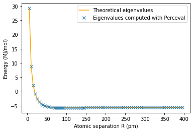
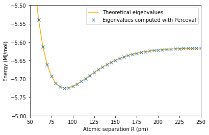
The minimum energy is E_g(0.9)=-5.725241527738244 MJ/mol and is attained for R_min =0.9 pm
Simulation n°2
[ ]:
tq = tqdm(desc='Minimizing...') #New progress bar
radius2=[]
E2=[]
init_param=[]

H=H2

for R in range(len(H)):            #We try to find the ground state eigenvalue for each radius R
    radius2.append(H[R][0])
    if (init_param==[]):           #
            init_param = [2*(np.pi)*random.random() for _ in List_Parameters]
    else:
        for i in range(len(init_param)):
            init_param[i]=VQE.get_parameters()[i]._value

    # Finding the ground state eigen value for each H(R)
    result=minimize(minimize_loss,init_param,method='Nelder-Mead')

    E2.append(result.get('fun'))
    tq.set_description('Finished' )
Simulation 2: computing the theoretical eigenvalues of H
We use the numpy linalg package.
[13]:
E2_th=[]
for h in H:
    l0=np.linalg.eigvals(h[1])
    l0.sort()
    E2_th.append(min(l0))
Simulation 2: plotting the results
The minimum eigenvalues of H are plotted in orange.
The eigenvalues found with Perceval are the crosses
[14]:
plt.plot(np.array(radius2),E2_th,'orange')
plt.plot(np.array(radius2),E2,'x')
plt.ylabel('Energy (MJ/mol)')
plt.xlabel('Atomic separation R (Å)')
plt.legend(['Theoretical eigenvalues', 'Eigenvalues computed with Perceval'])
plt.show()


plt.plot(np.array(radius2),E2_th,'orange')
plt.plot(np.array(radius2),E2,'x')
plt.axis([0.3,2,-1.2,-0.6])
plt.ylabel('Energy (MJ/mol)')
plt.xlabel('Atomic separation R (Å)')
plt.legend(['Theoretical eigenvalues', 'Eigenvalues computed with Perceval'])
plt.show()

min_value=min(E2)
min_index = E2.index(min_value)
print('The minimum energy is E_g('+str(radius2[min_index])+')='+str(E2[min_index])+' MJ/mol and is attained for R_min ='+str(radius1[min_index])+' Å')
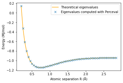
The minimum energy is E_g(0.75)=-1.1455991185105638 MJ/mol and is attained for R_min =0.6 Å
Simulation n°3
[ ]:
tq = tqdm(desc='Minimizing...') #New progress bar
radius3=[]
E3=[]
init_param=[]

H=H3

for R in range(len(H)):            #We try to find the ground state eigenvalue for each radius R
    radius3.append(H[R][0])
    if (init_param==[]):           #
            init_param = [2*(np.pi)*random.random() for _ in List_Parameters]
    else:
        for i in range(len(init_param)):
            init_param[i]=VQE.get_parameters()[i]._value

    # Finding the ground state eigen value for each H(R)
    result=minimize(minimize_loss,init_param,method='Nelder-Mead')

    E3.append(result.get('fun'))
    tq.set_description('Finished' )
Simulation 3: computing the theoretical eigenvalues of H
We use the numpy linalg package.
[16]:
E3_th=[]
for h in H:
    l0=np.linalg.eigvals(h[1])
    l0.sort()
    E3_th.append(min(l0))
Simulation 3: plotting the results
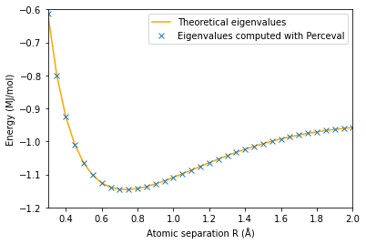
The minimum eigenvalue of H is plotted in orange.
The eigenvalues found with Perceval are the crosses
[17]:
plt.plot(np.array(radius3),E3_th,'orange')
plt.plot(np.array(radius3),E3,'x')
plt.ylabel('Energy (Hartree)')
plt.xlabel('Atomic separation R (Å)')
plt.legend(['Theoretical eigenvalues', 'Eigenvalues computed with Perceval'])
plt.show()


plt.plot(np.array(radius3),E3_th,'orange')
plt.plot(np.array(radius3),E3,'x')
plt.axis([0,2.5,-1.2,-0.6])
plt.ylabel('Energy (Hartree)')
plt.xlabel('Atomic separation R (Å)')
plt.legend(['Theoretical eigenvalues', 'Eigenvalues computed with Perceval'])
plt.show()

min_value=min(E3)
min_index = E3.index(min_value)
print('The minimum energy is E_g('+str(radius3[min_index])+')='+str(E3[min_index])+' Hartree and is attained for R_min ='+str(radius3[min_index])+' Å')
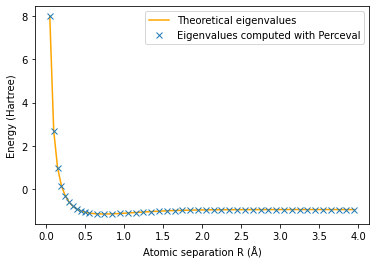
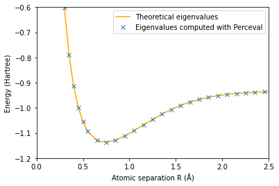
The minimum energy is E_g(0.75)=-1.1371172744346043 Hartree and is attained for R_min =0.75 Å
References
[1] A. Peruzzo, J. McClean, P. Shadbolt, M.-H. Yung, X.-Q. Zhou, P. J. Love,A. Aspuru-Guzik, and J. L. O’Brien, “A variational eigenvalue solver on a photonicquantum processor”, Nature Communications 5, 4213 (2014).
[2] P.J.J. O’Malley et al., “Scalable Quantum Simulation of Molecular Energies”, Phys. Rev. X 6, 031007 (2016)
[3] J.I. Colless, et al., “Computation of Molecular Spectra on a Quantum Processor with an Error-Resilient Algorithm”, Phys. Rev. X 8, 011021 (2018)
[4] J. A. Nelder and R. Mead, “A simplex method for function minimization”, The computer journal 7, 308–313 (1965).