You're reading the documentation of the v0.6. For the latest released version, please have a look at v0.11.

Circuits

Circuits Overview

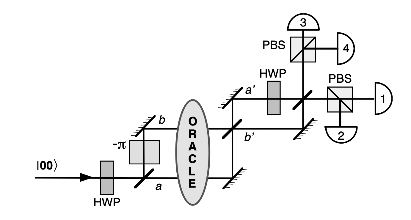
The concept of circuit is central in Perceval and the key component of the instrumentalist and the theoretician building a photonic quantum device. Perceval is giving concrete tools to reproduce an optical set-up in an optic laboratory with beams, mirrors and physical component but also photonic chips like a generic interferometer.

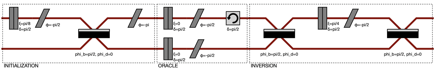
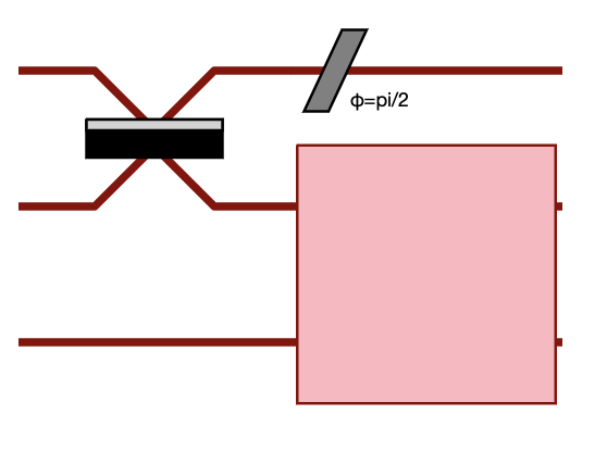
Optimized Grover algorithm as proposed in [Kwiat et al., 2000].	The equivalent circuit in Perceval
A 4-mode photonic chip (Copyright Quandela 2022)	The equivalent circuit in Perceval

What is a Circuit ?

In Perceval a circuit represents a setup of optical components, used to guide and act on photons.

A circuit has a fixed number of spatial modes (sometimes also called pathes or ports) \(m\), which is the same for input as for output spatial modes.

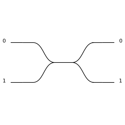
Simple examples of circuits are common optical devices such as beam splitters, phase shifters, or wave plates. Perceval provides a collection of these (see Components).

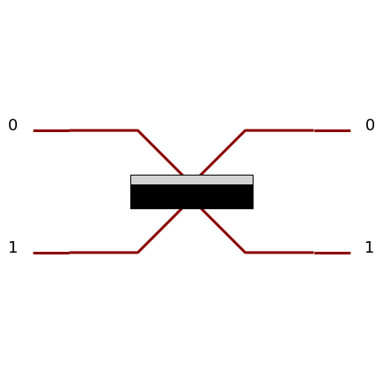
_images/bs.png — A beam splitter as a circuit in Perceval.

In particular, note that:

sources aren’t circuits, since they do not have input spatial modes (they don’t guide or act on incoming photons, but produce photons that are sent into a circuit),
detectors aren’t circuits either, for similar reasons

Warning

An optical circuit (just called “circuit” here) isn’t the same as a quantum circuit. Quantum circuits act on qubits, i.e. abstract systems in a 2-dimentional Hilbert space; while optical circuits act on photons distributed in spatial modes. It is possible to simply encode qubits with photons in an optical circuit; some encodings are presented in the Basics section.

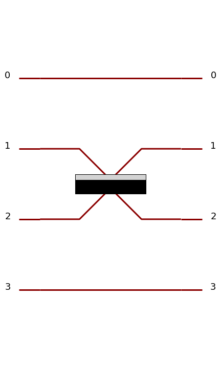
_images/basic-circuit.png — A simple circuit with 4 spatial modes, containing a beam splitter (being itself a circuit) between second and third spatial modes

Circuits can be combined together and used as building blocks to construct larger circuits. In the example above, a beam splitter, which is a builtin circuit with 2 spatial modes, has been used in a larger circuit with 4 spatial modes.

The lines, corresponding to spatial modes, are representing optical fibers on which photons are sent from the left to the right.

Building a Circuit

Each circuit corresponds to a Circuit object. To instantiate a circuit, simply pass the number of pathes as an argument:

>>> # create a new circuit with 3 spatial modes
>>> my_circuit = pcvl.Circuit(3)

Warning

Ports are using 0-based numbering - so port 0 is corresponding to the first line, … port \((m-1)\) is corresponding to the \(m\)-th line.

Predefined Circuits

Perceval provides two libraries of predefined circuits, named perceval.lib.phys and perceval.lib.symb (or shortly phys and symb):

>>> import perceval.lib.phys as phys
>>> import perceval.lib.symb as symb

These libraries contain simple circuits, which differ by their visual identities and specific mathematical definitions.

symb provides circuits with generally less parameters. This is useful to build generic optical circuits which implement quantum circuits, and perform symbolic computation.
phys provides circuits with more parameters, which allow a sharper modelisation of the components in a physical experiment.

For instance, the following table shows the respective definition of the unitary matrix of a beam splitter in the phys and the symb library:

Library	Definition	Representation
`symb`	\(\left[\begin{matrix}\cos{\left(\theta \right)} & i e^{- i \phi} \sin{\left(\theta \right)}\\i e^{i \phi} \sin{\left(\theta \right)} & \cos{\left(\theta \right)}\end{matrix}\right]\)
`phys`	\(\left[\begin{matrix}e^{i \phi_{a}} \cos{\left(\theta \right)} & i e^{i \phi_{b}} \sin{\left(\theta \right)}\\i e^{i \left(\phi_{a} - \phi_{b} + \phi_{d}\right)} \sin{\left(\theta \right)} & e^{i \phi_{d}} \cos{\left(\theta \right)}\end{matrix}\right]\)

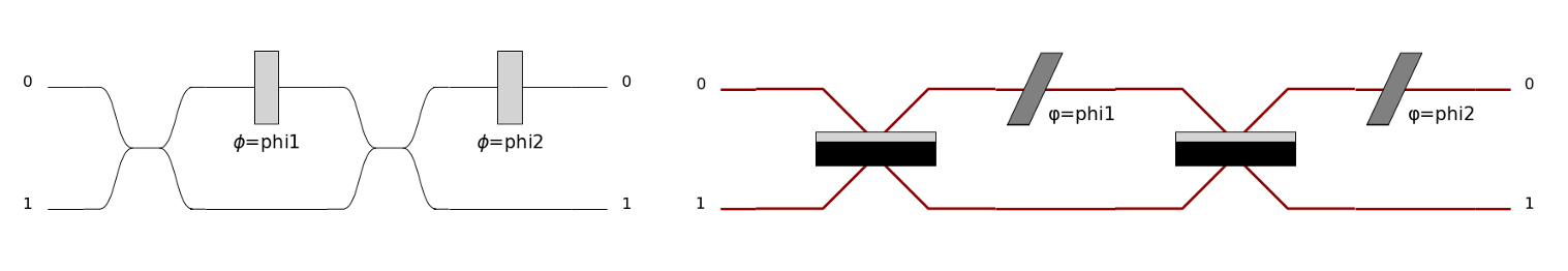
Also following figure shows the same Mach Zehnder Interferometer circuit represented with the symb and the phys library:

See Components for an overview of the circuits provided by symb and phys.

Tip

You can play with the python import namespace as to define a circuit without explicit reference to one or the other library. For instance, the following code defines a Mach Zehnder interferometer

>>> import perceval.lib.phys as plib
>>> mzi = (pcvl.Circuit(m=2, name="mzi")
...        .add((0, 1), plib.BS())
...        .add(0, plib.PS(pcvl.Parameter("phi1")))
...        .add((0, 1), plib.BS())
...        .add(0, plib.PS(pcvl.Parameter("phi2"))))

You would only need to change the first line to switch from one library to the other.

In addition to the generic properties of complex circuits, elementary circuits defined in phys and symb also have the following features:

Definition: definition() method gives the definition of the circuit - allowing to know in particular, the parameters to use and the way the unitary matrix is computed.
```
>>> pcvl.pdisplay(phys.BS().definition())
⎡cos(theta)               I*exp(-I*phi)*sin(theta)⎤
⎣I*exp(I*phi)*sin(theta)  cos(theta)              ⎦
```
Parameterization: most of the elementary circuits are defined by parameters. For instance a phase shifter will take the phase \(\phi\) as a parameter. You can either initialize these parameters with a fixed numeric value: phys.PS(1.57), with a symbolic value phys.PS(sp.pi/2) or with a non fixed parameter: phys.PS(pcvl.P("alpha")). See Parameters for more information.

Defining circuits from a unitary matrix

You can also define any circuit directly from a unitary matrix. In Perceval a unitary matrix corresponds to a Matrix object, which can simply created from a list matrix. The code:

>>> M = pcvl.Matrix([[0, 0, 1],
...                  [0, 1, 0],
...                  [1, 0, 0]])

corresponds to the unitary matrix: \(\left[\begin{matrix}0 & 0 & 1\\0 & 1 & 0\\1 & 0 & 0\end{matrix}\right]\)

The following then defines a circuit corresponding to this matrix:

>>> c1 = symb.Unitary(U=M)

You might also want to decompose the unitary matrix into a physical circuit using decomposition elements. Let us define for instance:

>>> ub = Circuit(2, name="ub") // symb.BS() // (0, symb.PS(phi=pcvl.Parameter("φ_a"))) // symb.BS() // (1, symb.PS(phi=pcvl.Parameter("φ_b")))

Then you can build a circuit using the method perceval.components.circuit.Circuit.decomposition():

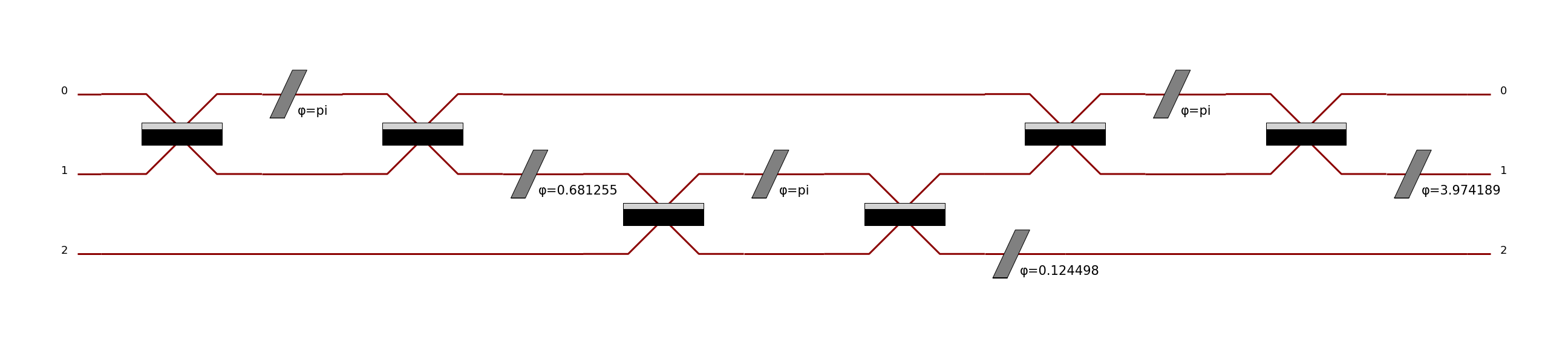
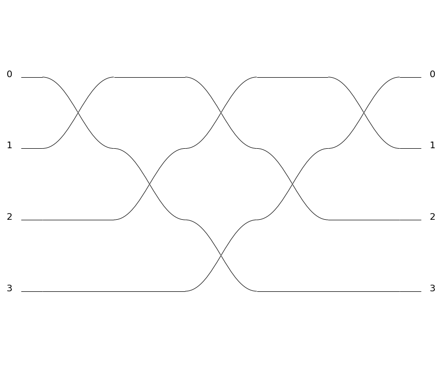
>>> c2 = pcvl.Circuit.decomposition(M, mzi, shape="triangle")
>>> c2.describe()
Circuit(3).add((0, 1), phys.BS()).add(0, phys.PS(phi=pi)).add((0, 1), phys.BS()).add(1, phys.PS(phi=0.681255)).add((1, 2), phys.BS()).add(1, phys.PS(phi=-pi)).add((1, 2), phys.BS()).add(2, phys.PS(phi=0.124498)).add((0, 1), phys.BS()).add(0, phys.PS(phi=pi)).add((0, 1), phys.BS()).add(1, phys.PS(phi=3.974189))
>>> pcvl.pdisplay(c2)

Some additional parameters can simplifiy the decomposition:

permutation: if set to a permutation component, permutations will be used when possible instead of a unitary block

>>> import perceval as pcvl
>>> import perceval.lib.symb as symb
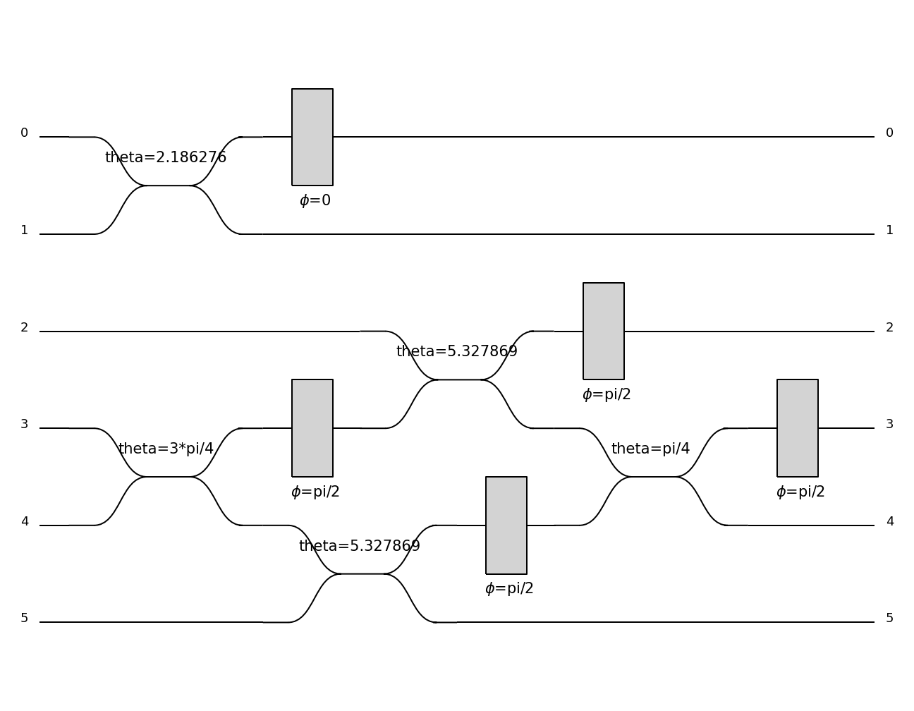
>>> C1 = pcvl.Circuit.decomposition(symb.PERM([3, 2, 1, 0]).compute_unitary(False),
>>>                                 symb.BS(theta=pcvl.Parameter("theta")),
>>>                                 permutation=symb.PERM,
>>>                                 shape="triangle")
>>>pcvl.pdisplay(C1)

constraints: you can provide a list of constraints on the different parameters of the unitary blocks to try to find circuits with constrained parameters. Each constraint is a t-uple of None or numerical value. When decomposing the circuit, the parameters will be searched iteratively in the constrained spaces. For instance: [(0, None), (np.pi/2, None), (None, None)] will allow to look for parameters pairs where the first parameter is 0 or \(pi/2\), or any value if no solution is found with the first constraints.

>>> U=1/3*np.array([[np.sqrt(3),-np.sqrt(6)*1j,0,0,0,0],
>>>                 [-np.sqrt(6)*1j,np.sqrt(3),0,0,0,0],
>>>                 [0,0,np.sqrt(3),-np.sqrt(3)*1j,-np.sqrt(3)*1j,0],
>>>                 [0,0,-np.sqrt(3)*1j,np.sqrt(3),0,np.sqrt(3)],
>>>                 [0,0,-np.sqrt(3)*1j,0,np.sqrt(3),-np.sqrt(3)],
>>>                 [0,0,0,np.sqrt(3),-np.sqrt(3),-np.sqrt(3)]])
>>> ub = symb.BS(theta=pcvl.P("theta"))//symb.PS(phi=pcvl.P("phi"))
>>> C1 = pcvl.Circuit.decomposition(U,
>>>                                 ub,
>>>                                 shape="triangle", constraints=[(None,0),(None,np.pi/2),
>>>                                                                (None,3*np.pi/2),(None,None)])

phase_shifter_fn: if you provide a phase-shifter to this parameter, the decomposition will add a layer of phases making the decomposed circuit strictly equivalent to the initial unitary matrix. In most cases, you can however omit this layer.
finally, you can also pass simpler unitary blocks - for instance a simple beamsplitter without phase, however in these cases, you might not obtain any solution in the decomposition

Complex Circuits

Assembling circuits

A circuit is defined by using Circuit object as following:

>>> c = pcvl.Circuit(m)

Where m is the number of modes of the circuit. See Circuit for additional parameters.

Then components of the circuit are added with the add primitive:

>>> c.add((0, 1), phys.BS())

Where:

The first parameter is either the port range (here ports 0 and 1), or the upper where the component should be added. The previous declaration is equivalent to:
```
>>> c.add(0, phys.BS())
```
The second parameter is a circuit, it can be an elementary circuit as in our example, or another complex circuit.

Tip

It is possible to add multiple components in a single statement allowing for simpler circuit declaration:

>>> mzi = pcvl.Circuit(2).add(0, plib.BS()).add(0, plib.PS(pcvl.Parameter("phi1")))\
...                      .add(0, plib.BS()).add(0, plib.PS(pcvl.Parameter("phi2"))))

alternatively, you can also use // notation for more compact definition, and start from unitary circuit:

>>> mzi = plib.BS() // (0, plib.PS(pcvl.Parameter("phi1"))) // plib.BS() // (0, plib.PS(pcvl.Parameter("phi2")))

Generic Interferometer

It is also possible to define generic interferometers with the static method perceval.components.circuit.Circuit.generic_interferometer().

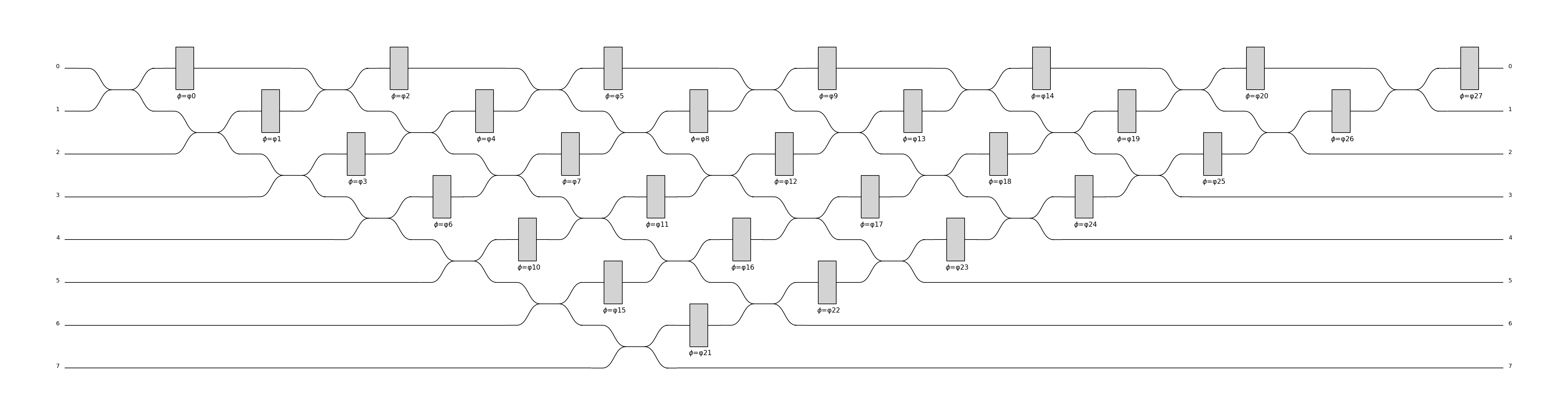
For instance the following defines a triangular interferometer on 8 modes using a beam splitter and a phase shifter as base components:

>>> c = pcvl.Circuit.generic_interferometer(8,
...                                         lambda i: symb.BS() // symb.PS(pcvl.P("φ%d" % i)),
...                                         shape="triangle")
>>> pcvl.pdisplay(c)

Sub-circuits

When you assemble to build a circuit, you can naturally include a complex circuit into another one:

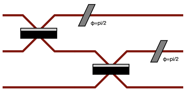
>>> bsps = phys.BS().add(0, phys.PS(sp.pi/2))
>>> c = pcvl.Circuit(3).add(0, bsps).add(1, bsps)
>>> pcvl.pdisplay(c)

By default, the new circuits merge all the circuits into a single one by using merge=False parameter:

>>> c = pcvl.Circuit(3).add(0, bsps).add(1, bsps, merge=False)
>>> pcvl.pdisplay(c)

This can be particularly useful to get a better visual organization of large circuit.

Unitary Matrices

Except for circuits using Time Delay, any circuit can be converted into its unitary matrix. Depending if your circuit is using Parameters or not, the unitary matrix will be symbolic or numeric.

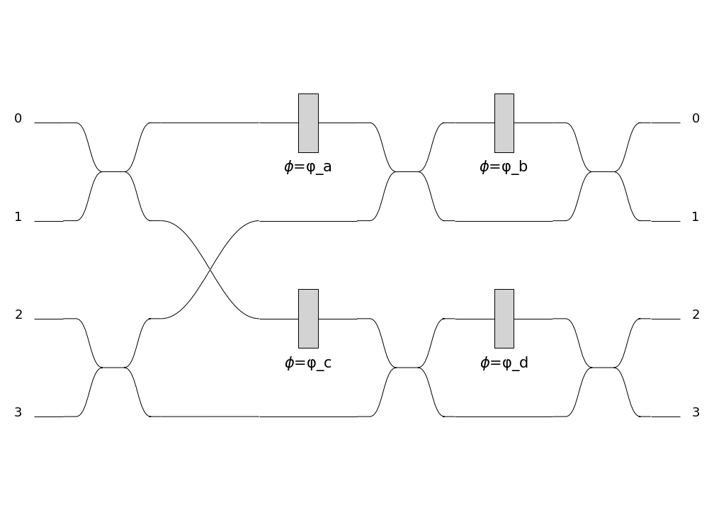
>>> chip4mode = pcvl.Circuit(m=4, name="QChip")
>>> phis = [pcvl.Parameter("phi1"), pcvl.Parameter("phi2"),
...         pcvl.Parameter("phi3"), pcvl.Parameter("phi4")]
>>> (chip4mode
...  .add((0, 1), symb.BS()).add((2, 3), symb.BS()).add((1, 2), symb.PERM([1, 0]))
...  .add(0, symb.PS(phis[0])).add(2, symb.PS(phis[2])).add((0, 1), symb.BS())
...  .add((2, 3), symb.BS()).add(0, symb.PS(phis[1])).add(2, symb.PS(phis[3]))
...  .add((0, 1), symb.BS()).add((2, 3), symb.BS()))
>>> pcvl.pdisplay(chip4mode.U)

\(\left[\begin{matrix}\frac{\sqrt{2} \left(- e^{i \phi_{1}} + e^{i \left(\phi_{1} + \phi_{2}\right)}\right)}{4} & \frac{\sqrt{2} i \left(- e^{i \phi_{1}} + e^{i \left(\phi_{1} + \phi_{2}\right)}\right)}{4} & \frac{\sqrt{2} i \left(e^{i \phi_{2}} + 1\right)}{4} & - \frac{\sqrt{2} \left(e^{i \phi_{2}} + 1\right)}{4}\\\frac{\sqrt{2} i \left(e^{i \phi_{1}} + e^{i \left(\phi_{1} + \phi_{2}\right)}\right)}{4} & - \frac{\sqrt{2} \left(e^{i \phi_{1}} + e^{i \left(\phi_{1} + \phi_{2}\right)}\right)}{4} & \frac{\sqrt{2} \left(1 - e^{i \phi_{2}}\right)}{4} & \frac{\sqrt{2} i \left(1 - e^{i \phi_{2}}\right)}{4}\\\frac{\sqrt{2} i \left(- e^{i \phi_{3}} + e^{i \left(\phi_{3} + \phi_{4}\right)}\right)}{4} & \frac{\sqrt{2} \left(- e^{i \phi_{3}} + e^{i \left(\phi_{3} + \phi_{4}\right)}\right)}{4} & - \frac{\sqrt{2} \left(e^{i \phi_{4}} + 1\right)}{4} & \frac{\sqrt{2} i \left(e^{i \phi_{4}} + 1\right)}{4}\\- \frac{\sqrt{2} \left(e^{i \phi_{3}} + e^{i \left(\phi_{3} + \phi_{4}\right)}\right)}{4} & \frac{\sqrt{2} i \left(e^{i \phi_{3}} + e^{i \left(\phi_{3} + \phi_{4}\right)}\right)}{4} & \frac{\sqrt{2} i \left(1 - e^{i \phi_{4}}\right)}{4} & \frac{\sqrt{2} \left(1 - e^{i \phi_{4}}\right)}{4}\end{matrix}\right]\)

See perceval.components.circuit.Circuit.compute_unitary() for more information.

Circuit Rewriting

To enable circuit rewriting operations introduced in [Clément et al., 2022], the following methods are available for matching a specific pattern in a circuit, and to replace the corresponding sub-circuit by an equivalent circuit.

The complete sequence is the following:

>>> while True:
...    # identify one instance of the parameterized "pattern" within a circuit
...    matched = circuit.match(pattern, browse=True)
...    # check if an occurence was found
...    if matched is None:
...       break
...    # transform the list of matched components into a sub-circuit
...    idx = a.isolate(list(matched.pos_map.keys()))
...    # check if an equivalent "rewrite" circuit can be found
...    res = optimize(rewrite, v, frobenius, sign=-1)
...    # check if we can rewrite this pattern closely enough to original circuit, here with frobenius distance
...    if res.fun > 1e-6:
...        break
...    # replace the subcircuit by a copy of the pattern
...    a.replace(idx, rewrite.copy(), merge=True)
...    # reset all parameters of pattern and rewrite circuit that have been instantiated by
...    # the matching/optimize process
...    pattern.reset_parameters()
...    rewrite.reset_parameters()

See Reference to Notebook for a complete functional example.