Density matrices in Fock space

In this notebook we introduce our new feature: density matrices in fock space. This space is a mathematical framework to describe the quantum states of a system with variable number of particles, photons in our case. Note that this space is much larger than the computational/logical space. Fock space is native to Perceval and hence these matrices can be indispensable for linear optic computations.

The difference in the basis is demonstrated in the following example of 1-qubit X gate. In logical space, the basic states of the system will be \(|0\rangle\), and \(|1\rangle\). The linear optical circuit implementation for this gate consists of a 2 mode circuit with the following basic states in the fock space - \(|00\rangle\), \(|10\rangle\), \(|01\rangle\), and, \(|11\rangle\).

We will demonstrate how to create density matrices in Perceval and the different methods can be applied on them for computation using @ simple examples - Bell State generation and Hong-Ou_Mandel effect.

import perceval as pcvl
import numpy as np
from perceval.components import BS, Source, Circuit, catalog
from perceval.utils import BasicState, DensityMatrix
from perceval import Simulator
from perceval.backends import SLOSBackend

Generating and Evolving a Bell State density matrix

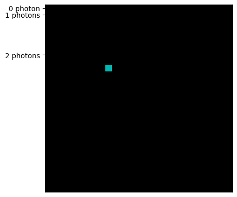
In Perceval, a density matrix is created by simply converting from the corresponding BasicState or StateVector Distribution.

input_dm = DensityMatrix.from_svd(BasicState([1,0,1,0,0,0]))
pcvl.pdisplay(input_dm)

The next step in applying the evolution operator is to define the LO circuit corresponding to the operation. Here, it is demonstrated by a Linear Optical circuit consisting of a Hadamard gate and a post-processed CNOT gate used for Bell State generation.

bell_circ = Circuit(m=6)

bell_circ.add(0, BS.H())
bell_circ.add(0, catalog['postprocessed cnot'].build_circuit(), merge=True)
pcvl.pdisplay(bell_circ)

To perform the computation on the input density matrix, a simulator is constructed with the circuit and the necessary post-selection function.

cnot = catalog['postprocessed cnot'].build_processor()  # creating a postprocessed cnot from catalog for the heralding and the post-selection function

bell_simulator = Simulator(SLOSBackend())
bell_simulator.set_circuit(bell_circ)
bell_simulator.set_selection(heralds=cnot.heralds, postselect=cnot.post_select_fn)

# Applying the evolution
bell_out_dm = bell_simulator.evolve_density_matrix(input_dm)  # apply evolution on the density matrix
print('Output Density matrix - Bell State')
pcvl.pdisplay(bell_out_dm)

Output Density matrix - Bell State

This output density matrix corresponds identically to evolving a statevector through the circuit and then converting the output SVD into a density matrix.

output_svd = bell_simulator.evolve(BasicState([1,0,1,0,0,0]))
print('The output statevector distribution:', output_svd)

print('The density matrix converted from the output SVD')
pcvl.pdisplay(DensityMatrix.from_svd(output_svd))

The output statevector distribution: sqrt(2)/2*|1,0,1,0,0,0>+sqrt(2)/2*|0,1,0,1,0,0>
The density matrix converted from the output SVD

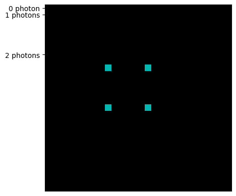
Investigating the Hong-Ou-Mandel effect using Density Matrix

For this we create a simulator with a 2 mode circuit consisting of a beam splitter. The output density matrix demonstrates quantum coherence through the non-zero off-diagonal coefficients.

sim = Simulator(SLOSBackend())
sim.set_circuit(BS.H())

# generate input density matrix
source = Source()  # perfect source
input_density_matrix = DensityMatrix.from_svd(source.generate_distribution(BasicState([1, 1])))

# evolution of density matrix
output_density_matrix = sim.evolve_density_matrix(input_density_matrix)
print('output density matrix without any loss')
pcvl.pdisplay(output_density_matrix)

output density matrix without any loss

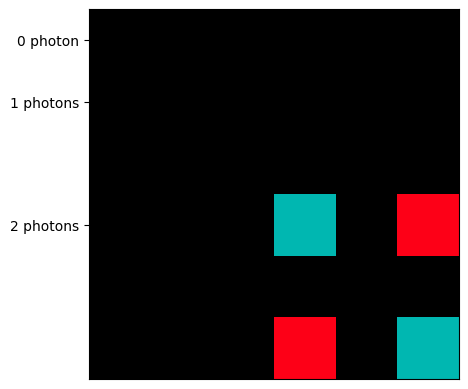
Apply a Loss operator on density matrix

The density matrices allow for application of a loss operator by defining the modes on which photons are lost and the probability of loss. The application of the loss operator and its effect are illustrated below using a simple 2 mode LO circuit with a beam splitter and a noisy source with emission probability of 0.6. Computationally, this is equivalent to a perfect source with a probaility of 0.4 for loosing a photon at each input mode before the circuit.

input_density_matrix.apply_loss([0, 1], 0.4)  # this loss operator is equivalent to 0.6 emission probability from source

lossy_output_density_matrix = sim.evolve_density_matrix(input_density_matrix)  # evolving this lossy density matrix
print('output density matrix with loss')
pcvl.pdisplay(lossy_output_density_matrix)

output density matrix with loss

Computing the expectation value of an operator

The expectation value of an operator \(\hat{O}\) over a quantum system represented by a density matrix \(\rho\) is given by the nice formula :

\[\langle\hat{O}\rangle = Tr (\hat{O}\rho)\]

In the next cell, we evaluate the expectation value of the number operator \(\hat{N}\) using the previous lossy density matrix generated by evolving through the beamsplitter.

dm_shape = lossy_output_density_matrix.shape

# Constructing the number operator
number_operator = np.zeros(dm_shape)
for state, index in lossy_output_density_matrix.index.items():
    number_operator[index, index] = state.n

expectation_value = (number_operator @ lossy_output_density_matrix.mat).trace()
print('The expectation value obtained (expected, there is a 60% chance of photons passing through the circuit):', expectation_value)

The expectation value obtained (expected, there is a 60% chance of photons passing through the circuit): (1.2000000000000004+0j)

Performing measurements on density matrix

A measurement on density matrix in Perceval is performed by defining the modes to be measured. The process returns a dictionary with the measured states as keys with values - probability of measuring the corresponding state and remaining density matrix. In T=the following cell, measurements on the output density matrix after the beam splitter (above) is demonstrated.

print('The output density matrix', output_density_matrix)

res = output_density_matrix.measure([0])  # performing measurements define the modes to measure
for keys, values in res.items():
    measured_state = keys
    prob_meas = values[0]
    remaining_dm = values[1]
    print('state measured:', measured_state, 'with probability', prob_meas, 'and the remaining density matrix', remaining_dm)

The output density matrix 0.50+0.00j*|2,0><2,0|+-0.50+0.00j*|0,2><2,0|+-0.50+0.00j*|2,0><0,2|+0.50+0.00j*|0,2><0,2|
state measured: |0> with probability 0.5000000000000001 and the remaining density matrix 1.00+0.00j*|2><2|
state measured: |2> with probability 0.5000000000000001 and the remaining density matrix 1.00+0.00j*|0><0|

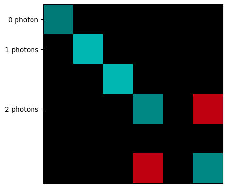
Let’s see the difference if this measurement was performed on the lossy case

print('The lossy output density matrix', lossy_output_density_matrix)

lossy_res = lossy_output_density_matrix.measure([0])  # choose modes to measure
for keys, values in lossy_res.items():
    print('state measured:', keys, 'with probability', values[0])  # key: measured basic state, values[0]: probability of measuring the state

The lossy output density matrix 0.16+0.00j*|0,0><0,0|+0.24+0.00j*|1,0><1,0|+0.00+0.00j*|0,1><1,0|+0.00+0.00j*|1,0><0,1|+0.24+0.00j*|0,1><0,1|+0.18+0.00j*|2,0><2,0|+-0.18+0.00j*|0,2><2,0|+-0.18+0.00j*|2,0><0,2|+0.18+0.00j*|0,2><0,2|
state measured: |0> with probability 0.5800000000000002
state measured: |1> with probability 0.24000000000000005
state measured: |2> with probability 0.18000000000000008