You're reading the documentation of the v1.0. For the latest released version, please have a look at v1.2.
pdisplay
Also known as “Perceval pretty display”, is a generic function designed to display a lot of different types of Perceval objects.
This method has two variants:
pdisplaythat displays the object immediately. The format and place of output might depend on where your code is executed (IDE, notebook…) and the kind of object that is displayed.pdisplay_to_filethat doesn’t display the object but saves its representation in a file specified by a string path. This method always usesFormat.MPLOT(for matplotlib) by default, so you might need to specify it by hand it for some objects.
Display a circuit
Any circuit coded in perceval can be displayed. You just need to make the code associated with the desired circuit, let’s call it circ, and add pcvl.pdisplay(circ) afterwards in the python cell. Note that components follow the same rules than circuits for displaying.
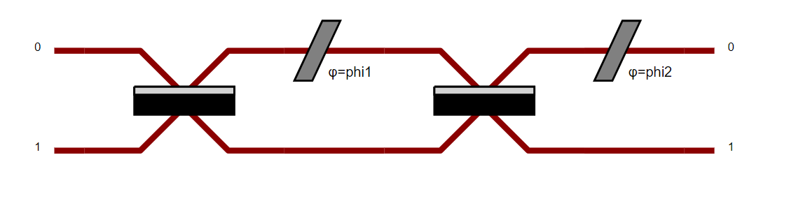
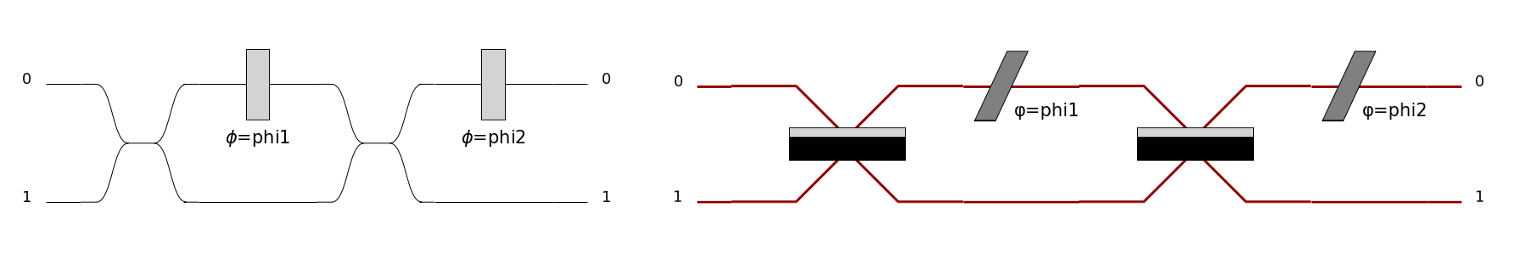
Let’s do an example to understand: you want to display the Mach-Zendher Interferometer.
Start by doing the code associated to the circuit.
import perceval.components.unitary_components as comp

mzi = (pcvl.Circuit(m=2, name="mzi")
      .add((0, 1), comp.BS())
      .add(0, comp.PS(pcvl.Parameter("phi1")))
      .add((0, 1), comp.BS())
      .add(0, comp.PS(pcvl.Parameter("phi2"))))
Then, add pcvl.pdisplay() of your circuit.
pcvl.pdisplay(mzi)
Tip
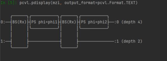
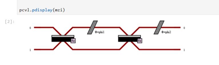
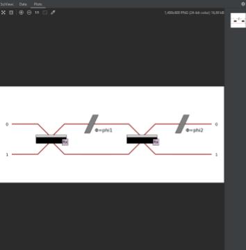
The outcome of this last command will depend on your environment.
Text Console |
Jupyter Notebook |
IDE (Pycharm, Spyder, etc) |
|---|---|---|
|
|
|
Controlling the circuit rendering
Also, you can change the display of the circuit using a different skin which can itself be configured. Indeed, a boolean can be set to obtain a more compact display (if the circuit is too wide for example).
import perceval as pcvl
import perceval.components.unitary_components as comp
from perceval.rendering.circuit import SymbSkin
C = pcvl.Circuit.decomposition(pcvl.Matrix(comp.PERM([3, 1, 0, 2]).U),
comp.BS(R=pcvl.P("R")), phase_shifter_fn=comp.PS)
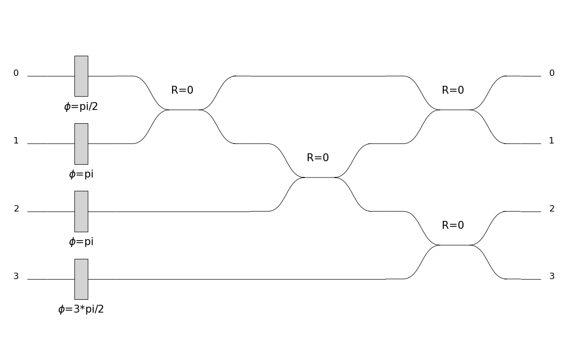
symbolic_skin = SymbSkin(compact_display=True)
pcvl.pdisplay(C, skin=symbolic_skin)
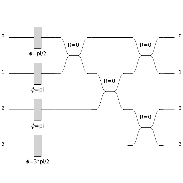
symbolic_skin = SymbSkin(compact_display=False)
pcvl.pdisplay(C, skin=symbolic_skin)
By default the skin will be PhysSkin, if you want to use another skin by default, you can save your configuration
into your Perceval persistent configuration. Currently, the other skin provided with Perceval is SymbSkin:
To save the skin in your configuration, you need to use the DisplayConfig object.
The possible kwargs when displaying a Circuit are
output_format. The format to use for the output, from thePerceval.Formatenum. The available formats are MPLOT (default), TEXT and LATEX.recursive. IfTrue, the first layer of inner circuits will be exposed in the rendering.compact. If no skin is provided, the skin taken from theDisplayConfigwill have this value forcompact_displayprecision. The numerical precision to display.nsimplify. IfTrue(default), some values will be displayed with known mathematical values (pi, sqrt, fractions) if close enoughskin. The skin to use. If none is provided, the skin from theDisplayConfigwill be used.
Display a Processor
Like circuits, Processor can also be displayed using pdisplay.
Note that the behaviour is strictly the same for Experiment and RemoteProcessor.
For a Processor containing only a circuit, the result is the same as for displaying a Circuit.
However, some objects defined in the Processor will also be displayed if defined, modifying the look of the results.
Every object that can be named will display its name near to where it is shown.
We take the same example as before for this demonstration.
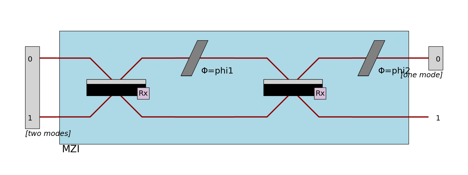
Ports
When defined, ports are represented by encapsulating the mode numbers in rectangles.
>>> proc = pcvl.Processor("SLOS", mzi)
>>> proc.add_port(0, pcvl.Port(pcvl.Encoding.DUAL_RAIL, "two modes"), location=pcvl.PortLocation.INPUT)
>>> proc.add_port(0, pcvl.Port(pcvl.Encoding.RAW, "one mode"), location=pcvl.PortLocation.OUTPUT)
>>> pcvl.pdisplay(proc, recursive=True)
Detectors
When defined, detectors are displayed at the right of the circuit with different shapes to be more recognizable:
PNR detectors are represented by a half-circle
PPNR detectors are represented by a polygon
threshold detectors are represented by a triangle
>>> proc = pcvl.Processor("SLOS", 3).add(0, mzi)
>>> proc.add(0, pcvl.Detector.pnr())
>>> proc.add(1, pcvl.Detector.ppnr(24))
>>> proc.add(2, pcvl.Detector.threshold())
>>> pcvl.pdisplay(proc, recursive=True)
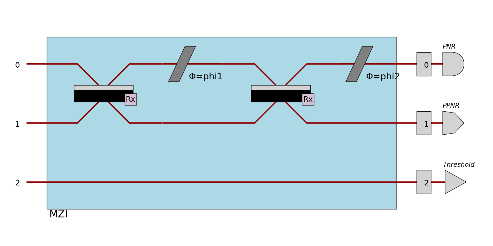
Notice that in that case, the mode number is shown as if there was a single-mode port.
Also, if there are components after detectors (such as feed-forward configurators), the color of the optical path will change to indicate that this mode is now a classical mode.
Heralds
When defined, heralds are displayed using half-circles with their value inside the circle. Also, they hide a part of the optical path to be as close as possible to the components they are used in. The modes numbers on which the heralds are defined are not shown.
>>> proc = pcvl.Processor("SLOS", mzi)
>>> proc.with_input(pcvl.BasicState([1, 0]))
>>> pcvl.pdisplay(proc, recursive=True)
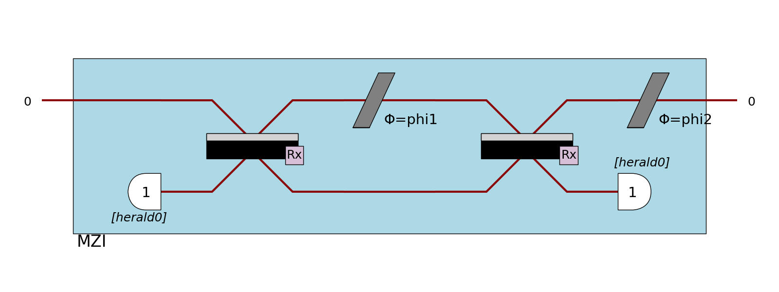
In case a detector is defined on the same mode than an herald, the half-circle is replaced by the shape of the detector. Notice that for PNR detectors, the shape doesn’t change, but the number of expected photons is added into the half-circle.
Input state
If possible, the photons of the input state will be displayed at the left of the processor.
This is globally the case when the input state is a BasicState, and the processor is displayed in a SVG format.
>>> proc = pcvl.Processor("SLOS", mzi)
>>> proc.with_input(pcvl.BasicState([1, 0]))
>>> pcvl.pdisplay(proc, recursive=True)
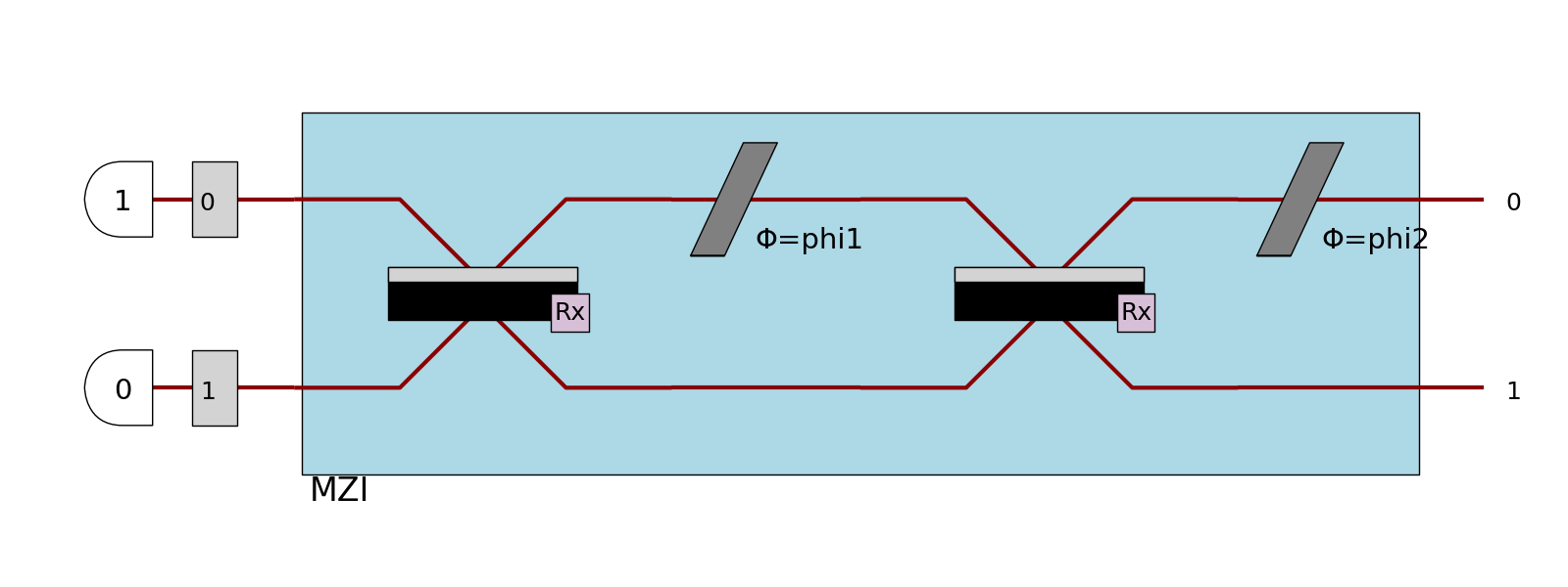
Notice that in this case, the modes are displayed as if they had a single-mode port (if no port is defined), and the photons are displayed like heralds except that they don’t hide the mode.
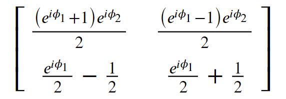
Displaying a Matrix
Matrices, both numeric and symbolic, can be displayed using pdisplay
>>> m = Matrix([[1, 2], ["x/2", np.pi]], use_symbolic=True)
>>> pcvl.pdisplay(m)
⎡1    2 ⎤
⎣x/2  pi⎦
The possible kwargs when displaying a Matrix are
output_format. The format to use for the output, from theperceval.Formatenum. The available formats are TEXT (default), and LATEX.precision. The numerical precision to display numbers.
Using pdisplay on a pcvl.Matrix is a simple way to include a LaTex rendering in a document.
Displaying a DensityMatrix
Density matrices are displayed differently than regular matrices.
Instead of a table, pdisplay uses matplotlib to represent them using a 2d plot where pixels represent the amplitudes of different states.
See Density matrices in Fock space
The possible kwargs when displaying a DensityMatrix are:
color. IfTrue(default), the result is a color image where colors represent the phase of the states.cmap. Any colormap from matplotlib as a str to use to represent the phase of the states.
Displaying a distribution
StateVector, BSCount, BSDistribution and SVDistribution
can be displayed in a table format using pdisplay,
the behaviour being similar for all these classes.
All of them are normalized before being displayed.
>>> state = pcvl.StateVector([1, 0]) + 1j * pcvl.StateVector([0, 1])
>>> pcvl.pdisplay(state)
+-------+-------------+
| state | prob. ampl. |
+-------+-------------+
| |1,0> |  sqrt(2)/2  |
| |0,1> | I*sqrt(2)/2 |
+-------+-------------+
The main use of this display is that it can sort the keys by value and display only a limited number of keys, allowing the display to be fast and to keep only the most important information.
>>> bsd = pcvl.BSDistribution({pcvl.BasicState([0]): 0.1, pcvl.BasicState([1]): 0.7, pcvl.BasicState([2]): 0.2})
>>> pcvl.pdisplay(bsd, max_v=2)  # Sort by default, keep only the 2 highest values
+-------+-------------+
| state | probability |
+-------+-------------+
|  |1>  |    7/10     |
|  |2>  |     1/5     |
+-------+-------------+
The possible kwargs when displaying a StateVector, BSCount, BSDistribution or SVDistribution are
output_format. The format to use for the output, from thePerceval.Formatenum. The available formats are TEXT (default), LATEX and HTML.nsimplify. IfTrue(default), some values will be displayed with known mathematical values (pi, sqrt, fractions) if close enough. However, if the distribution to be displayed is too large and if this parameter is not manually set toTrue, this numerical simplification will be unactivated.precision. The numerical precision to display numbers.max_v. The number of values to display.sort. IfTrue(default), values will be sorted before being displayed.
Displaying samples
BSSamples can be displayed in a table format using pdisplay.
>>> bs_samples = pcvl.BSSamples()
>>> bs_samples.append(perceval.BasicState("|1,0>"))
>>> bs_samples.append(perceval.BasicState("|1,1>"))
>>> bs_samples.append(perceval.BasicState("|0,1>"))
>>> pcvl.pdisplay(bs_samples)
+--------+
| states |
+--------+
| |1,0>  |
| |1,1>  |
| |0,1>  |
+--------+
The number of displayed states can be limited with the parameter max_v.
>>> pcvl.pdisplay(bs_samples, max_v=2)  # keep only the 2 first values
+--------+
| states |
+--------+
| |1,0>  |
| |1,1>  |
+--------+
The possible kwargs when displaying a BSSamples are
output_format. The format to use for the output, from thePerceval.Formatenum. The available formats are TEXT (default), LATEX and HTML.max_v. The number of values to display.max_vis 10 by default.
Displaying algorithms
Some algorithms can be passed to pdisplay to display their results easily.
Analyzer
In the case of the Analyzer, it displays the results as a table, as well as the performance and fidelity of the gate.
See usage in Ralph CNOT Gate.
The possible kwargs when displaying an Analyzer are:
output_format. The format to use for the output, from thePerceval.Formatenum. The available formats are TEXT (default), LATEX and HTML.nsimplify. IfTrue(default), some values will be displayed with known mathematical values (pi, sqrt, fractions) if close enoughprecision. The numerical precision to display numbers.
Tomography
In the case of a tomography algorithm, it displays the results as a table, as well as the performance and fidelity of the gate. See usage in Tomography of a CNOT Gate.
The possible kwargs when displaying a tomography algorithm are:
precision. The numerical precision to display numbers.render_size. The size to create the matplotlib figure.
Display a JobGroup
pdisplay can be used to represent a JobGroup.
The result is a table showing a resume of the status of the jobs inside the job group.
>>> jg = pcvl.JobGroup("example")  # Result might change depending on what is in this group
>>> pcvl.pdisplay(jg)
+--------------+-------+--------------------------------------+
| Job Category | Count |               Details                |
+--------------+-------+--------------------------------------+
|    Total     |   8   |                                      |
|   Finished   |   5   | {'successful': 4, 'unsuccessful': 1} |
|  Unfinished  |   3   |      {'sent': 1, 'not sent': 2}      |
+--------------+-------+--------------------------------------+
The possible kwargs when displaying a tomography algorithm are:
output_format. The format to use for the output, from thePerceval.Formatenum. The available formats are TEXT (default), LATEX and HTML.
Display a graph
pdisplay offers support to quickly display graphs from nx.graph.
The possible kwargs when displaying a graph are:
output_format. The format to use for the output, from thePerceval.Formatenum. The available formats are MPLOT (default), and LATEX.
Code reference
- perceval.rendering.pdisplay.pdisplay(o, output_format=None, **opts)
Pretty display Main rendering entry point. Several data types can be displayed using pdisplay.
- Parameters:
o – Perceval object to render
output_format (
Optional[Format]) – Format controls where and how a figure is render (in a interactive window, the terminal, etc.) - MPLOT: Matplotlib drawing (default in IDE - spyder, pycharm or vscode) - HTML: HTML for data table, SVG for circuits/processors (default in notebook) - TEXT: Pretty text display (default in another cases) - LATEX: LaTex code, drawing with Tikz for circuits/processors
- opts:
skin (rendering.circuit.PhysSkin, SymbSkin or DebugSkin or any ASkin subclass instance):
Skin controls how a circuit/processor is displayed:
PhysSkin(): physical skin (default),
DebugSkin(): Similar to PhysSkin but modes are bigger, ancillary modes are displayed, components with variable parameters are red,
SymbSkin(): symbolic skin (thin black and white lines).
precision (float): numerical precision
nsimplify (bool): if True, tries to simplify numerical values by searching known values (pi, sqrt, fractions)
recursive (bool): if True, all hierarchy levels in a circuit/processor are displayed. Otherwise, only the top level is drawn, others are “black boxes”
max_v (int): Maximum number of displayed values in distributions
sort (bool): if True, sorts a distribution (descending order) before displaying
render_size: In SVG circuit/processor rendering, acts as a zoom factor (float) In Tomography display, is the size of the output plot in inches (tuple of two floats)
- perceval.rendering.pdisplay.pdisplay_to_file(o, path, output_format=None, **opts)
Directly saves the result of pdisplay into a file without actually displaying it.
- Parameters:
o – Perceval object to render
path (
str) – Path to file to saveoutput_format (
Optional[Format]) – Seepdisplayfor details. Contrarily topdisplay, this method always uses Format.MPLOT by default so you might need to specify it by hand for some kinds of objects.opts – See
pdisplayfor details.
- enum perceval.rendering.format.Format(value)
Enum class used to specify the output format of pdisplay. The possible formats depend on the object type to render.
Valid values are as follows:
- TEXT = <Format.TEXT: 1>
Text output, suitable for display in a terminal.
- MPLOT = <Format.MPLOT: 2>
Use the Matplotlib engine, opens its own graphic window or shows in an IDE graph view.
- HTML = <Format.HTML: 3>
Outputs HTML compatible code: SVG for images, <table> for a table of data, etc.
- LATEX = <Format.LATEX: 4>
Outputs LaTex code.