CHSH experiment
In this notebook, we aim to reproduce the \(\mathsf{CNOT}\) Gate to evaluate its performance while demonstrating key features of Perceval. We use as basis the implementation from [1].
[1]:
import math

import perceval as pcvl
Ralph CNOT Gate
We start by building the circuit as defined by the paper above - it is a circuit on six modes (labelled from 0 to 5 from top to bottom) consisting of five beam splitters. Modes 0 and 1 contain the control system while modes 2 and 3 encode the target system. Modes 4 and 5 are unoccupied ancillary modes (they are not displayed, but they are required).
[2]:
p = pcvl.catalog['postprocessed cnot'].build_experiment()

pcvl.pdisplay(p, recursive=True)
[2]:
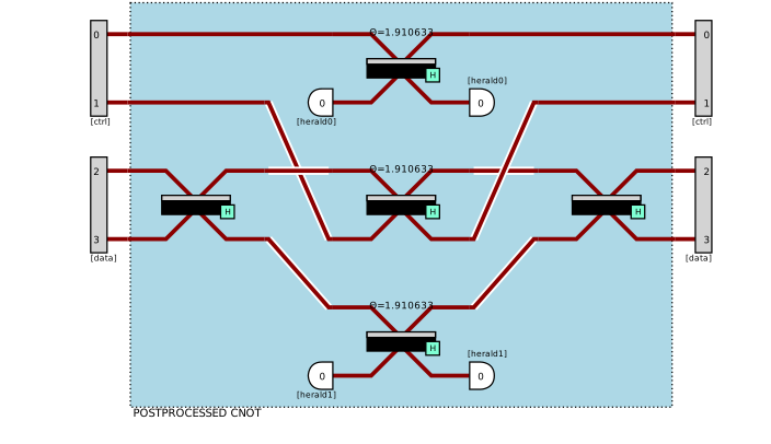
Simulations will run on this circuit, using four different input states corresponding to the two-qubit computational basis states. The Analyzer is used to compute the gate performance.
[3]:
states = {
    pcvl.BasicState([1, 0, 1, 0]): "00",
    pcvl.BasicState([1, 0, 0, 1]): "01",
    pcvl.BasicState([0, 1, 1, 0]): "10",
    pcvl.BasicState([0, 1, 0, 1]): "11"
}

computer = pcvl.SimulatedComputer("SLOS")
with computer.acquire():
    ca = pcvl.algorithm.Analyzer(computer, p, states)
    ca.compute(expected={"00": "00", "01": "01", "10": "11", "11": "10"})
pcvl.pdisplay(ca)
print(f"performance = {pcvl.simple_float(ca.performance)[1]}, fidelity = {ca.fidelity * 100}%")
| 00 | 01 | 10 | 11 | |
|---|---|---|---|---|
| 00 | 1 | 0 | 0 | 0 |
| 01 | 0 | 1 | 0 | 0 |
| 10 | 0 | 0 | 0 | 1 |
| 11 | 0 | 0 | 1 | 0 |
performance = 1/9, fidelity = 100.0%
Beyond the actual logic function, what is interesting with this gate us that it produces entangled states that we will be trying to check with CHSH experiment when the source is not perfect.
Checking for entanglement with CHSH experiment
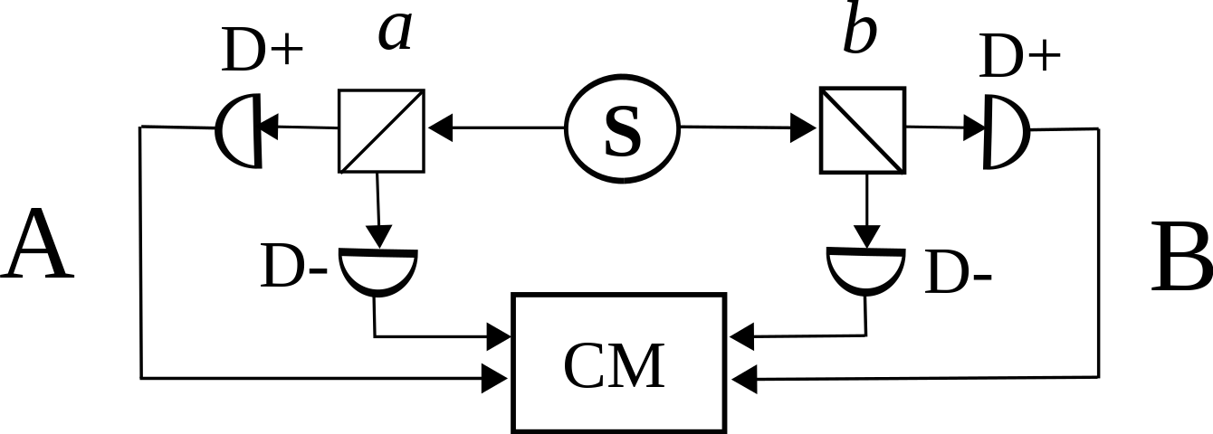 https://en.wikipedia.org/wiki/File:Two_channel_bell_test.svg
To reproduce this Bell test protocol, we define a new experiment that uses the \(\mathsf{CNOT}\) gate implemented above as a sub-experiment. The parameters \(a\) and \(b\) describe the measurement bases used by players \(A\) and \(B\). A noise model with a brightness of 40% and a purity of 99% is assigned to the simulated computer.
[4]:
noise = pcvl.NoiseModel(brightness=0.4, g2=0.01)

experiment = pcvl.Experiment(4)
experiment.add(0, pcvl.BS.H())
experiment.add(0, p)

a = pcvl.Parameter("a")
b = pcvl.Parameter("b")

experiment.add(0, pcvl.BS.H(theta=a))
experiment.add(2, pcvl.BS.H(theta=b))

pcvl.pdisplay(experiment, recursive=True)
[4]:
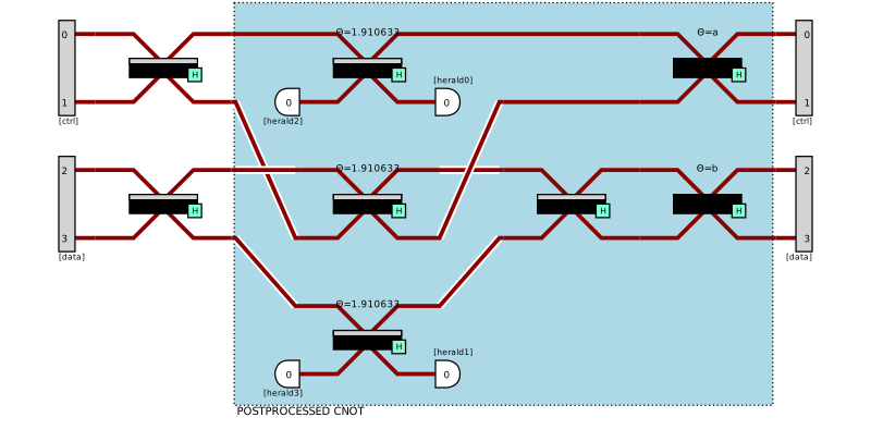
We start by setting the values of the two parameters to 0, meaning that the beam splitters after the \(\mathsf{CNOT}\) effectively act as the identity.
[5]:
a.set_value(0)
b.set_value(0)
We now state that our photons will be inputted on ports 0 and 2 (using the 0-index convention, and not counting heralded modes).
[6]:
experiment.min_detected_photons_filter(2)
experiment.with_input(pcvl.BasicState([1, 0, 1, 0]))
We now detail the different state vectors that form the probabilistic source input. The most frequent input is the empty state, followed by two states with only one photon on either input port, then by the nominal input \(|1,0,1,0,0,0\rangle\). Heralded modes are included because their photons are subject to the same imperfect source. They appear at the end of the state because they were added after the experiment was declared.
[7]:
source = pcvl.Source.from_noise_model(noise)
source_distribution = source.generate_distribution(pcvl.BasicState([1, 0, 1, 0, 0, 0]))
pcvl.pdisplay(source_distribution, precision=1e-4)
| state | probability |
|---|---|
| |0,0,0,0,0,0> | 9/25 |
| |{0},0,0,0,0,0> | 0.2395 |
| |0,0,{0},0,0,0> | 0.2395 |
| |{0},0,{0},0,0,0> | 0.1594 |
| |0,0,{0}{4},0,0,0> | 4.8193e-4 |
| |{0}{2},0,0,0,0,0> | 4.8193e-4 |
| |{0},0,{0}{4},0,0,0> | 3.2064e-4 |
| |{0}{2},0,{0},0,0,0> | 3.2064e-4 |
| |{0}{2},0,{0}{4},0,0,0> | 0 |
We can then check the output state distribution corresponding to this input distribution. By default, since our input state had 2 photons, only states having at least 2 detected photons are kept. This can be changed using min_detected_photons_filter.
[8]:
computer = pcvl.SimulatedComputer("SLOS")
computer.noise = noise
factory = pcvl.ExecutionFactory(computer, experiment)

with computer.acquire():
    output_distribution = factory.probs()["results"]
pcvl.pdisplay(output_distribution, max_v=10)
| state | probability |
|---|---|
| |0,1,0,1> | 0.495518 |
| |1,0,1,0> | 0.495518 |
| |0,1,1,0> | 0.00747 |
| |1,0,0,1> | 0.001494 |
Let us run now the experiment with increasing value of g2 in the range \([0, 0.2]\) with a brightness of \(0.15\) and check the CHSH inequality.
[9]:
from tqdm.auto import tqdm
import numpy as np

x = np.arange(0, 20, 0.5)
y = []

with computer.acquire():
    for g2 in tqdm(x):
        Es = []
        for va in [0, math.pi / 2]:
            a.set_value(va)
            for vb in [math.pi / 4, 3 * math.pi / 4]:
                b.set_value(vb)
                Npp, Npm, Nmp, Nmm = 0, 0, 0, 0
                computer.noise = pcvl.NoiseModel(brightness=0.15, g2=g2 / 100)
                output_distribution = factory.probs()["results"]
                for output_state, prob in output_distribution.items():
                    if output_state[0] == 1 and output_state[2] == 1:
                        Npp = prob
                    if output_state[0] == 1 and output_state[3] == 1:
                        Npm = prob
                    if output_state[1] == 1 and output_state[2] == 1:
                        Nmp = prob
                    if output_state[1] == 1 and output_state[3] == 1:
                        Nmm = prob
                E = (Npp - Npm - Nmp + Nmm) / (Npp + Npm + Nmp + Nmm)
                Es.append(E)

        S = Es[0] - Es[1] + Es[2] + Es[3]
        print(f"g2 = {g2 / 100}, S = {S}")
        y.append(S)
g2 = 0.0, S = 2.8284271247461903
g2 = 0.005, S = 2.792615361258137
g2 = 0.01, S = 2.7572980402457263
g2 = 0.015, S = 2.7224649920120614
g2 = 0.02, S = 2.6881063238088334
g2 = 0.025, S = 2.6542124105426095
g2 = 0.03, S = 2.6207738857392098
g2 = 0.035, S = 2.5877816329598575
g2 = 0.04, S = 2.5552267774696427
g2 = 0.045, S = 2.5231006783080483
g2 = 0.05, S = 2.4913949206290438
g2 = 0.055, S = 2.4601013083623045
g2 = 0.06, S = 2.4292118571395154
g2 = 0.065, S = 2.3987187875083835
g2 = 0.07, S = 2.368614518400099
g2 = 0.075, S = 2.338891660848145
g2 = 0.08, S = 2.3095430119332683
g2 = 0.085, S = 2.28056154897453
g2 = 0.09, S = 2.251940423920364
g2 = 0.095, S = 2.22367295795931
g2 = 0.1, S = 2.19575263631623
g2 = 0.105, S = 2.1681731032549507
g2 = 0.11, S = 2.140928157249369
g2 = 0.115, S = 2.114011746338283
g2 = 0.12, S = 2.0874179636398176
g2 = 0.125, S = 2.0611410430335115
g2 = 0.13, S = 2.035175354988402
g2 = 0.135, S = 2.00951540254766
g2 = 0.14, S = 1.9841558174433025
g2 = 0.145, S = 1.9590913563550196
g2 = 0.15, S = 1.9343168972953646
g2 = 0.155, S = 1.9098274361218837
g2 = 0.16, S = 1.885618083164027
g2 = 0.165, S = 1.8616840599720907
g2 = 0.17, S = 1.838020696169706
g2 = 0.175, S = 1.8146234264183836
g2 = 0.18, S = 1.7914877874790276
g2 = 0.185, S = 1.7686094153746597
g2 = 0.19, S = 1.7459840426455244
g2 = 0.195, S = 1.7236074956965992
[10]:
import matplotlib.pyplot as plt
plt.title("CHSH value with purity")
plt.xlabel("g2 (%)")
plt.ylabel("Bell inequality")
plt.axhline(y=2, linewidth=2, color="red", label='horizontal-line')
plt.plot(x, y, color ="green")
plt.grid(color='b', dashes=(3, 2, 1, 2))
plt.show()
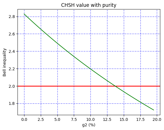
Beyond 13% of g2, we are crossing the value \(2\), i.e. not violating anymore the \(|CHSH|\le 2\) inequality!
Reference
[1] T. C. Ralph, N. K. Langford, T. B. Bell, and A. G. White. Linear optical controlled-NOT gate in the coincidence basis. Physical Review A, 65(6):062324, June 2002. Publisher: American Physical Society.