Graph States

I. Some definitions and properties of graph states

Graph states are specific entangled states that are represented by a graph. They have interesting properties in many fields of quantum computing [1], therefore they are points of interest.

Definition

Two definitions of a graph state exist. Since they are equivalent, we will only consider the following:

Given a graph \(G=(V,E)\), with the set of vertices \(V\) and the set of edges \(E\), the corresponding graph state is defined as:

\(\left|G\right\rangle = \prod_{(a,b)\in E} CZ^{\{a,b\}} \left|+\right\rangle^{\otimes V}\)

where \(|+\rangle = \frac{|0\rangle + |1\rangle}{\sqrt2}\) and \(CZ^{\{a,b\}}\) is the controlled-Z interaction between the two vertices (corresponding to two qubits) \(a\) and \(b\). The operators order in the product doesn’t matter since CZ gates commute between themselves. We can write the CZ gate with the following matrix :

\(CZ = \begin{bmatrix} 1 & 0 & 0 & 0 \\ 0 & 1 & 0 & 0 \\ 0 & 0 & 1 & 0 \\ 0 & 0 & 0 & -1 \\ \end{bmatrix}\)

Therefore, we can write the action of a CZ gate as: \(CZ^{\{1,2\}}|0\rangle_1 |\pm\rangle_2 = |0\rangle_1 |\pm\rangle_2\) and \(CZ^{\{1,2\}}|1\rangle_1 |\pm\rangle_2 = |1\rangle_1 |\mp\rangle_2\).

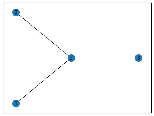
Let’s illustrate this with an example. The associated graph of: \(|\Psi_{graph}\rangle = CZ^{\{0,1\}}\, CZ^{\{1,2\}}\, CZ^{\{0,2\}}\, CZ^{\{3,2\}}|+\rangle_0 |+\rangle_1 |+\rangle_2 |+\rangle_3\) is the following. The graph is generated as an output later in this notebook. We will now see several ways to create and display these states.

II. Generating entangled states with a circuit

We will first use a 3-qubits circuit. We need to implement two CZ gates on it to generate the 3-qubits linear graph state.

These gates are post-selected CZ gates which have a probability of success of \(\frac{1}{9}\).

import math
import perceval as pcvl
import networkx as nx
from perceval.utils import StateGenerator, Encoding

Implementation in Perceval

For this circuit, we use path encoded qubits with 3 photons as input.

# Modes number of the circuit
m = 10

# Creation of the full circuit
cz = pcvl.catalog["postprocessed cz"].build_circuit()

c_graph_lin = pcvl.Circuit(10, name="C_Graph")\
    .add((1, 2), pcvl.BS()).add(1, pcvl.PS(math.pi/2))\
    .add((3, 4), pcvl.BS()).add(3, pcvl.PS(math.pi/2))\
    .add((7, 8), pcvl.BS()).add(7, pcvl.PS(math.pi/2))\
    .add(0, cz, merge=False)\
    .add((3,4,5,6), pcvl.PERM([2, 3, 0, 1]))\
    .add(4, cz, merge=False)\
    .add(8, pcvl.PS(math.pi/2)).add(7, pcvl.PS(math.pi/2))\
    .add((3,4,5,6), pcvl.PERM([2, 3, 0, 1]))

pcvl.pdisplay(c_graph_lin, recursive=True, render_size=0.6)

Logical states

Logical states are path encoded on the Fock States.

Due to post-selection, only few states of the full Fock space are relevant.

• Mode 0,5,6,9 are auxiliary.

• 1st qubit is path encoded in modes 1 & 2

• 2nd qubit in 3 & 4

• 3rd qubit in 7 & 8

# Basis for three qubits
states = [
    pcvl.BasicState([0,1,0,1,0,0,0,1,0,0]),  #|000>
    pcvl.BasicState([0,1,0,1,0,0,0,0,1,0]),  #|001>
    pcvl.BasicState([0,1,0,0,1,0,0,1,0,0]),  #|010>
    pcvl.BasicState([0,1,0,0,1,0,0,0,1,0]),  #|011>
    pcvl.BasicState([0,0,1,1,0,0,0,1,0,0]),  #|100>
    pcvl.BasicState([0,0,1,1,0,0,0,0,1,0]),  #|101>
    pcvl.BasicState([0,0,1,0,1,0,0,1,0,0]),  #|110>
    pcvl.BasicState([0,0,1,0,1,0,0,0,1,0])   #|111>
]

Computation of the output state

We will then simulate this circuit using the SLOS backend and compute the amplitudes for the output state.

# Simulator
backend = pcvl.BackendFactory.get_backend("SLOS")
backend.set_circuit(c_graph_lin)

We use the state \(|000\rangle\) as input state.

# Input state
input_state = pcvl.BasicState([0, 1, 0, 1, 0, 0, 0, 1, 0, 0])
backend.set_input_state(input_state)

# Output state
output_state = pcvl.StateVector()
for state in states:
    ampli = backend.prob_amplitude(state)
    output_state += ampli*pcvl.StateVector(state)

print("The output state is :", output_state)

The output state is : 0.118*|0,0,1,0,1,0,0,1,0,0>-0.118*|0,1,0,1,0,0,0,1,0,0>-0.02*|0,1,0,0,1,0,0,0,1,0>+0.118*|0,1,0,1,0,0,0,0,1,0>+0.687*|0,0,1,1,0,0,0,0,1,0>+0.02*|0,1,0,0,1,0,0,1,0,0>-0.687*|0,0,1,1,0,0,0,1,0,0>-0.118*|0,0,1,0,1,0,0,0,1,0>

As wanted, we obtain the linear graph states for three qubits which is : \(\frac{1}{\sqrt 8} (|000\rangle + |001\rangle + |010\rangle - |011\rangle + |100\rangle + |101\rangle - |110\rangle + |111\rangle )\).

This state is also locally equivalent to a \(GHZ\) state and we can therefore obtain it by performing local unitary single qubit transformations. To visualize this state using plot_state_qsphere from Qiskit [2] or plot_schmidt from qutip [3], follow the StatevectorConverter example from perceval-interop [4].

III. Generate a state from a graph

We also developed a tool which takes as input a graph from networkx and provides the associated graph state.

# Create the graph with networkx
G = nx.Graph()
G.add_nodes_from([2,1,0,3])

G.add_edge(0,1)
G.add_edge(1,2)
G.add_edge(2,0)
G.add_edge(2,3)

nx.draw_networkx(G, with_labels=True)

We choose the encoding type we want.

# Set the generator with the dual rail encoding
generator = StateGenerator(Encoding.DUAL_RAIL)

Then we use the generator to create the graph state:

graph_state = generator.graph_state(G)
print(graph_state)

0.25*|0,1,1,0,1,0,1,0>+0.25*|1,0,0,1,0,1,0,1>+0.25*|1,0,1,0,1,0,1,0>+0.25*|1,0,0,1,1,0,1,0>-0.25*|0,1,1,0,0,1,1,0>-0.25*|0,1,0,1,1,0,1,0>+0.25*|1,0,1,0,0,1,1,0>-0.25*|1,0,0,1,0,1,1,0>-0.25*|0,1,0,1,0,1,1,0>+0.25*|0,1,1,0,1,0,0,1>+0.25*|1,0,1,0,1,0,0,1>-0.25*|0,1,0,1,1,0,0,1>+0.25*|1,0,0,1,1,0,0,1>+0.25*|0,1,1,0,0,1,0,1>-0.25*|1,0,1,0,0,1,0,1>+0.25*|0,1,0,1,0,1,0,1>

You can use the generated state as an input state in any noiseless simulation

p = pcvl.Processor("SLOS", pcvl.Unitary(pcvl.Matrix.random_unitary(8)))  # Use a 8x8 random unitary matrix as a circuit
p.min_detected_photons_filter(4)
p.with_input(graph_state)
sampler = pcvl.algorithm.Sampler(p)
pcvl.pdisplay(sampler.probs()['results'], max_v=10)

state	probability
|1,0,1,1,1,0,0,0>	0.018002
|0,0,0,1,2,1,0,0>	0.015395
|0,0,0,0,0,0,4,0>	0.015104
|0,0,0,0,1,3,0,0>	0.015061
|1,1,0,0,2,0,0,0>	0.014839
|1,0,0,1,0,0,0,2>	0.013904
|0,0,0,0,1,2,0,1>	0.011317
|0,1,0,1,0,0,2,0>	0.011303
|1,0,0,0,0,1,2,0>	0.011015
|1,2,0,0,0,1,0,0>	0.010701

References

[1] Marc Hein et al. “Entanglement in graph states and its applications”. In: arXiv preprint quant-ph/0602096 (2006). https://arxiv.org/abs/quant-ph/0602096

[2] https://qiskit.org/documentation/stubs/qiskit.visualization.plot_state_qsphere.html

[3] https://nbviewer.org/urls/qutip.org/qutip-tutorials/tutorials-v4/visualization/qubism-and-schmidt-plots.ipynb

[4] https://perceval.quandela.net/interopdocs/